- The Inverted Multi-Index

Содержание
- 2. From images to descriptors
- 3. Query process Dataset of visual descriptors Image set: Query: Important extras: + geometric verification + query
- 4. Demands Initial setup: Dataset size: few million images Typical RAM size: few dozen gigabytes Tolerable query
- 5. Meeting the demands Main observation: the vectors have a specific structure: correlated dimensions, natural image statistics,
- 6. The inverted index Sivic & Zisserman ICCV 2003
- 7. Querying the inverted index Have to consider several words for best accuracy Want to use as
- 8. Product quantization [Jegou, Douze, Schmid // TPAMI 2011]: Split vector into correlated subvectors use separate small
- 9. The inverted multi-index Our idea: use product quantization for indexing Main advantage: For the same K,
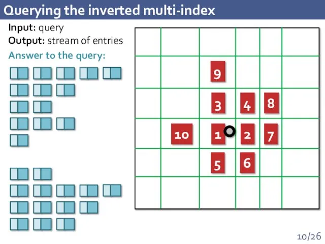
- 10. Querying the inverted multi-index 1 2 3 4 5 6 7 8 9 10 Input: query
- 11. Querying the inverted multi-index – Step 1
- 12. Querying the inverted multi-index – Step 2 1 2 3 4 5 6 1 2 3
- 13. Querying the inverted multi-index
- 14. Experimental protocol Dataset: 1 billion of SIFT vectors [Jegou et al.] Hold-out set of 10000 queries,
- 15. Performance comparison Recall on the dataset of 1 billion of visual descriptors: 100x Time increase: 1.4
- 16. Performance comparison Recall on the dataset of 1 billion 128D visual descriptors:
- 17. Time complexity For same K index gets a slight advantage because of BLAS instructions
- 18. Memory organization Overhead from multi-index: Averaging over N descriptors:
- 19. Why two? For larger number of parts: Memory overhead becomes larger Population densities become even more
- 20. Multi-Index + Reranking "Multi-ADC": use m bytes to encode the original vector using product quantization "Multi-D-ADC":
- 21. Multi-ADC vs. Exhaustive search
- 22. Multi-D-ADC vs State-of-the-art State-of-the-art [Jegou et al.] Combining multi-index + reranking:
- 23. Performance on 80 million GISTs Multi-D-ADC performance: Index vs Multi-index: Same protocols as before, but on
- 24. Retrieval examples Exact NN Uncompressed GIST Multi-D-ADC 16 bytes Exact NN Uncompressed GIST Multi-D-ADC 16 bytes
- 25. Multi-Index and PCA (128->32 dimensions)
- 26. Conclusions A new data structure for indexing the visual descriptors Significant accuracy boost over the inverted
- 27. Other usage scenarios Large-scale NN search' based approaches: Holistic high dimensional image descriptors: GISTs, VLADs, Fisher
- 29. Скачать презентацию
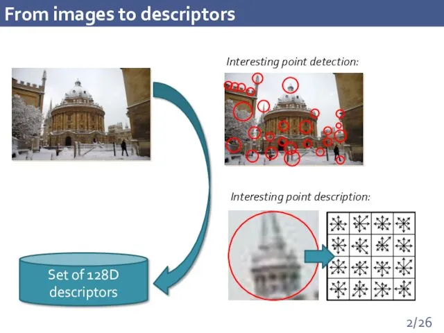
From images to descriptors
From images to descriptors
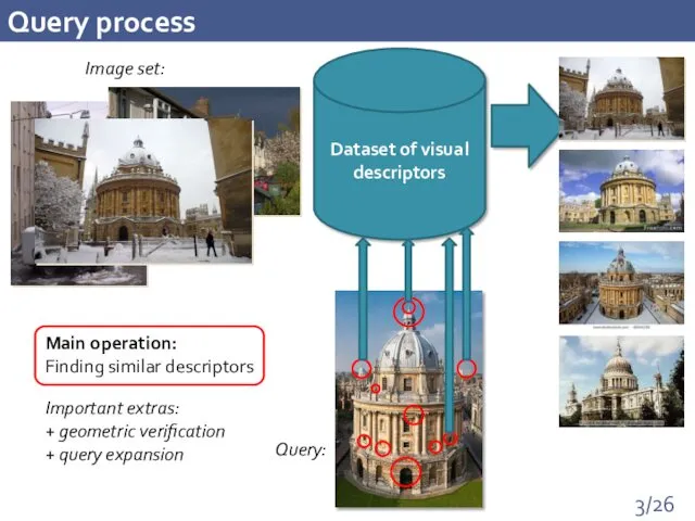
Query process
Dataset of visual descriptors
Image set:
Query:
Important extras:
+ geometric verification
+ query expansion
Main
Query process
Dataset of visual descriptors
Image set:
Query:
Important extras:
+ geometric verification
+ query expansion
Main
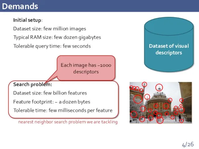
Demands
Initial setup:
Dataset size: few million images
Typical RAM size: few dozen gigabytes
Tolerable
Demands
Initial setup:
Dataset size: few million images
Typical RAM size: few dozen gigabytes
Tolerable
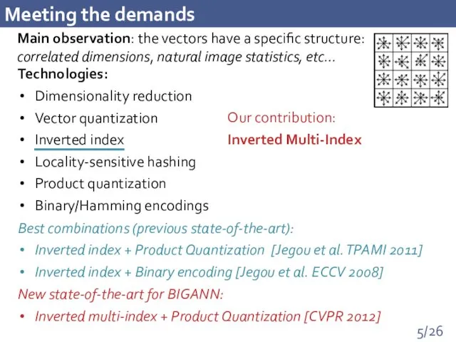
Meeting the demands
Main observation: the vectors have a specific structure: correlated
Meeting the demands
Main observation: the vectors have a specific structure: correlated
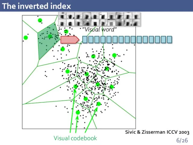
The inverted index
Sivic & Zisserman ICCV 2003
The inverted index
Sivic & Zisserman ICCV 2003
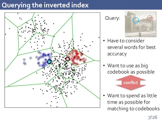
Querying the inverted index
Have to consider several words for best accuracy
Want
Querying the inverted index
Have to consider several words for best accuracy
Want
![Product quantization [Jegou, Douze, Schmid // TPAMI 2011]: Split vector](/_ipx/f_webp&q_80&fit_contain&s_1440x1080/imagesDir/jpg/87883/slide-7.jpg)
Product quantization
[Jegou, Douze, Schmid // TPAMI 2011]:
Split vector into correlated subvectors
use
Product quantization
[Jegou, Douze, Schmid // TPAMI 2011]:
Split vector into correlated subvectors
use
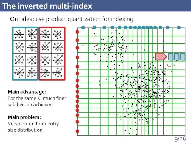
The inverted multi-index
Our idea: use product quantization for indexing
Main advantage:
For
The inverted multi-index
Our idea: use product quantization for indexing
Main advantage:
For
Querying the inverted multi-index
1
2
3
4
5
6
7
8
9
10
Input: query
Output: stream of entries
Answer to the query:
Querying the inverted multi-index
1
2
3
4
5
6
7
8
9
10
Input: query
Output: stream of entries
Answer to the query:
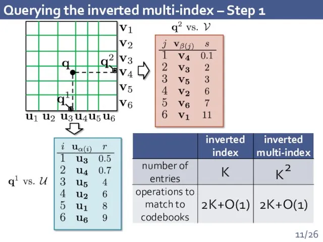
Querying the inverted multi-index – Step 1
Querying the inverted multi-index – Step 1
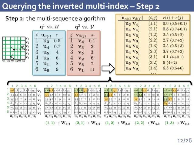
Querying the inverted multi-index – Step 2
1
2
3
4
5
6
1
2
3
4
5
6
1
2
3
4
5
6
1
2
3
4
5
6
1
2
3
4
5
6
1
2
3
4
5
6
Step 2: the multi-sequence algorithm
Querying the inverted multi-index – Step 2
1
2
3
4
5
6
1
2
3
4
5
6
1
2
3
4
5
6
1
2
3
4
5
6
1
2
3
4
5
6
1
2
3
4
5
6
Step 2: the multi-sequence algorithm
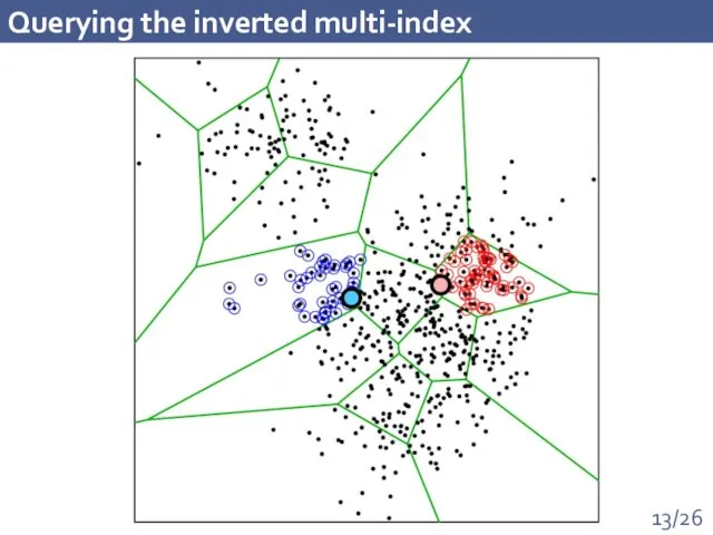
Querying the inverted multi-index
Querying the inverted multi-index
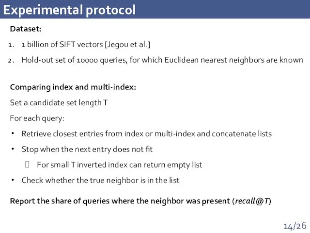
Experimental protocol
Dataset:
1 billion of SIFT vectors [Jegou et al.]
Hold-out set
Experimental protocol
Dataset:
1 billion of SIFT vectors [Jegou et al.]
Hold-out set
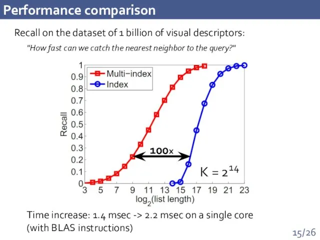
Performance comparison
Recall on the dataset of 1 billion of visual descriptors:
100x
Time
Performance comparison
Recall on the dataset of 1 billion of visual descriptors:
100x
Time
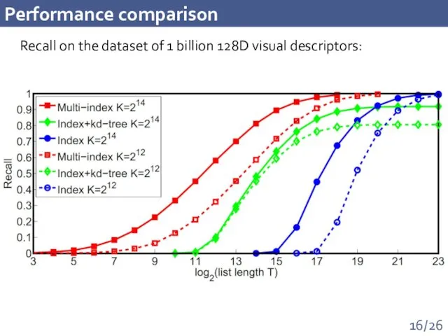
Performance comparison
Recall on the dataset of 1 billion 128D visual descriptors:
Performance comparison
Recall on the dataset of 1 billion 128D visual descriptors:
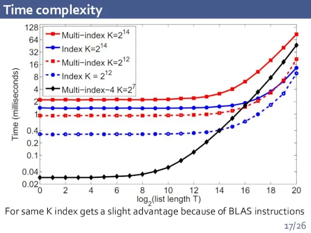
Time complexity
For same K index gets a slight advantage because of
Time complexity
For same K index gets a slight advantage because of
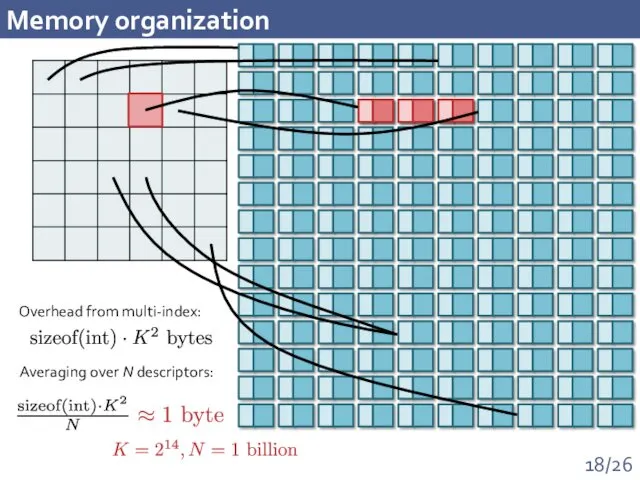
Memory organization
Overhead from multi-index:
Averaging over N descriptors:
Memory organization
Overhead from multi-index:
Averaging over N descriptors:
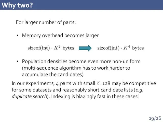
Why two?
For larger number of parts:
Memory overhead becomes larger
Population densities become
Why two?
For larger number of parts:
Memory overhead becomes larger
Population densities become
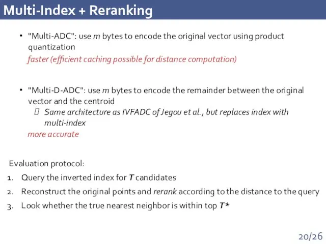
Multi-Index + Reranking
"Multi-ADC": use m bytes to encode the original vector
Multi-Index + Reranking
"Multi-ADC": use m bytes to encode the original vector
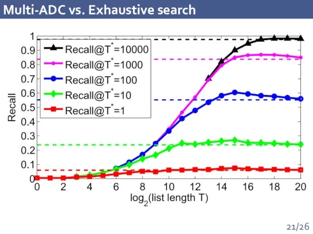
Multi-ADC vs. Exhaustive search
Multi-ADC vs. Exhaustive search
![Multi-D-ADC vs State-of-the-art State-of-the-art [Jegou et al.] Combining multi-index + reranking:](/_ipx/f_webp&q_80&fit_contain&s_1440x1080/imagesDir/jpg/87883/slide-21.jpg)
Multi-D-ADC vs State-of-the-art
State-of-the-art [Jegou et al.]
Combining multi-index + reranking:
Multi-D-ADC vs State-of-the-art
State-of-the-art [Jegou et al.]
Combining multi-index + reranking:
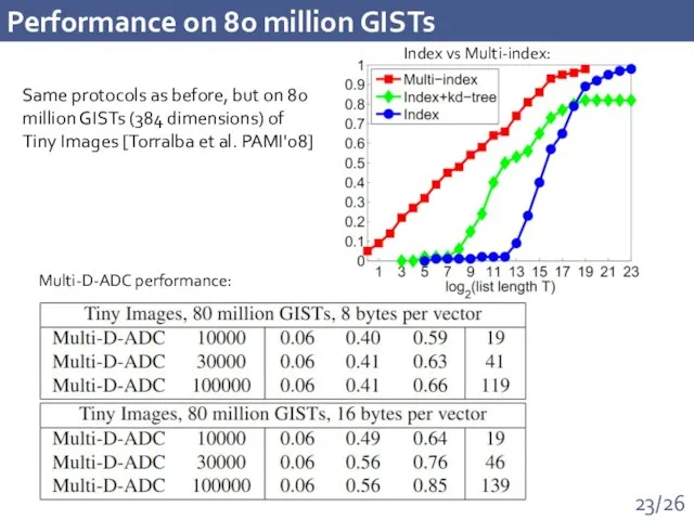
Performance on 80 million GISTs
Multi-D-ADC performance:
Index vs Multi-index:
Same protocols as before,
Performance on 80 million GISTs
Multi-D-ADC performance:
Index vs Multi-index:
Same protocols as before,
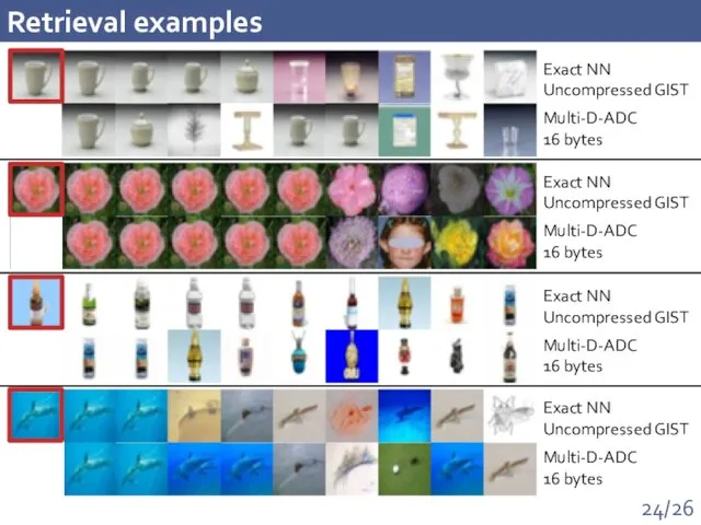
Retrieval examples
Exact NN
Uncompressed GIST
Multi-D-ADC
16 bytes
Exact NN
Uncompressed GIST
Multi-D-ADC
16 bytes
Exact NN
Uncompressed GIST
Multi-D-ADC
16 bytes
Exact
Retrieval examples
Exact NN
Uncompressed GIST
Multi-D-ADC
16 bytes
Exact NN
Uncompressed GIST
Multi-D-ADC
16 bytes
Exact NN
Uncompressed GIST
Multi-D-ADC
16 bytes
Exact
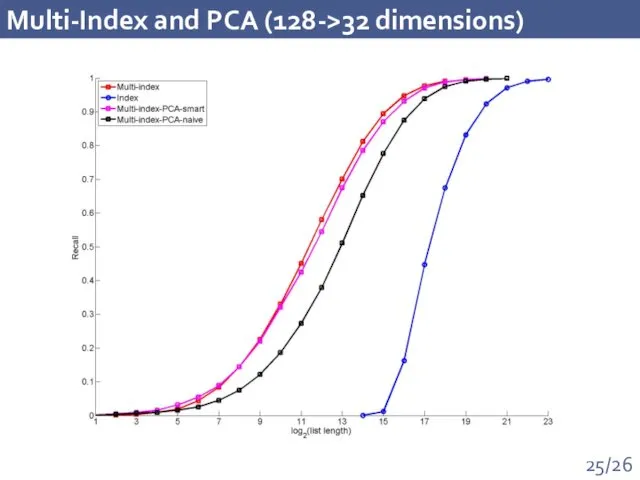
Multi-Index and PCA (128->32 dimensions)
Multi-Index and PCA (128->32 dimensions)
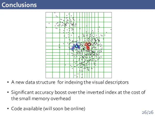
Conclusions
A new data structure for indexing the visual descriptors
Significant accuracy
Conclusions
A new data structure for indexing the visual descriptors
Significant accuracy
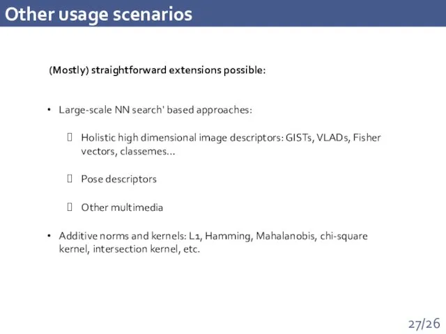
Other usage scenarios
Large-scale NN search' based approaches:
Holistic high dimensional image
Other usage scenarios
Large-scale NN search' based approaches:
Holistic high dimensional image
 Как подготовить данные. Семинар 4. Викторина
 Концепция и возможности подхода .NET
 Microsoft Access Мәліметтер қорын басқару жүйесі
 Технология создания и обработки графической информации
 Презентация Времена года. 6 класс
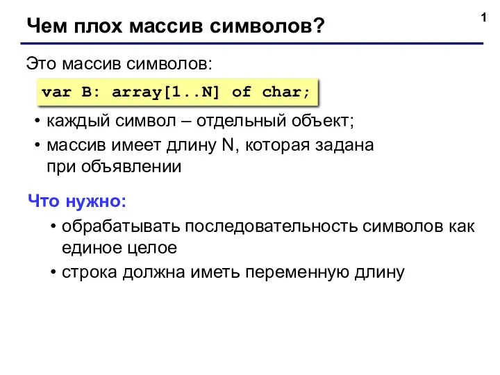 Строки Паскаль. Чем плох массив символов?
 Научная информация: поиск, накопление и обработка
 Обслуживание сети
 Introduction to Data Capture. Module 6
 Решение логических задач
 Передача информации. Приложение к уроку
 Добровольцы России. Регистрация организации
 Упрощение логических выражений. Решение задач
 ВКР: Совершенствование системы управления персоналом сервисного предприятия
 Как снимать интересные сториз
 Память. Что такое память компьютера
 Практические аспекты составления алгоритмов
 Теоретические основы информатики
 Информационные технологии в государственном управлении
 Компьютерлік желі
 WEB. Visual Studio Code
 Браузеры. Яндекс Браузер, Opera, Firefox
 SQL. База данных
 Системы управления базами данных (СУБД) MS Access
 Решение задач с использованием операторов цикла
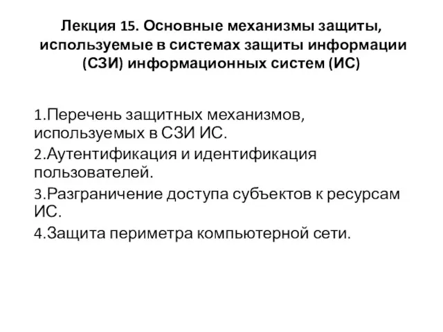 Лекция 15. Основные механизмы защиты, используемые в системах защиты информации (СЗИ) информационных систем (ИС)
 Графический учебный исполнитель. Разработка урока с презентацией
 Программирование на языке Java. Тема 23. Рекурсия