- Correlation Regression

Содержание
- 2. Causation
- 3. Causation Causation is any cause that produces an effect. This means that when something happens (cause)
- 4. Correlation Correlation measures the relationship between two things. Positive correlations happen when one thing goes up,
- 5. Correlation Correlations happen when: A causes B B causes A A and B are consequences of
- 6. Causation and Correlation Causation and correlation can happen at the same time. But having a correlation
- 7. Correlation or Causation? As people’s happiness level increases, so does their helpfulness. This would be a
- 8. Correlation or Causation? Dogs pant to cool themselves down. This would be a causation. When a
- 9. Correlation or Causation? Among babies, those who are held more tend to cry less. This would
- 10. Let's think of our own Correlation: Causation:
- 11. Quick Review Causation is any cause that produces an effect. Correlation measure the relationship between two
- 12. Correlation
- 13. The Question Are two variables related? Does one increase as the other increases? e. g. skills
- 14. Scatterplots Graphically depicts the relationship between two variables in two dimensional space.
- 15. Direct Relationship
- 16. Inverse Relationship
- 17. An Example Does smoking cigarettes increase systolic blood pressure? Plotting number of cigarettes smoked per day
- 18. Trend?
- 19. Smoking and BP Note relationship is moderate, but real. Why do we care about relationship? What
- 20. Heart Disease and Cigarettes Data on heart disease and cigarette smoking in 21 developed countries Data
- 21. The Data Surprisingly, the U.S. is the first country on the list--the country with the highest
- 22. Scatterplot of Heart Disease CHD Mortality goes on Y axis Why? Cigarette consumption on X axis
- 23. {X = 6, Y = 11}
- 24. What Does the Scatterplot Show? As smoking increases, so does coronary heart disease mortality. Relationship looks
- 25. Correlation Co-relation The relationship between two variables Measured with a correlation coefficient Most popularly seen correlation
- 26. Types of Correlation Positive correlation High values of X tend to be associated with high values
- 27. Correlation Coefficient A measure of degree of relationship. Between 1 and -1 Sign refers to direction.
- 29. Covariance The formula for co-variance is: How this works, and why? When would covXY be large
- 30. Example
- 31. Example What the heck is a covariance? I thought we were talking about correlation?
- 32. Correlation Coefficient Pearson’s Product Moment Correlation Symbolized by r Covariance ÷ (product of the 2 SDs)
- 33. Calculation for Example CovXY = 11.12 sX = 2.33 sY = 6.69
- 34. Example Correlation = .713 Sign is positive Why? If sign were negative What would it mean?
- 35. Factors Affecting r Range restrictions Looking at only a small portion of the total scatter plot
- 36. Factors Affecting r Outliers Overestimate Correlation Underestimate Correlation
- 37. Countries With Low Consumptions
- 38. Outliers
- 39. Testing Correlations So you have a correlation. Now what? In terms of magnitude, how big is
- 40. Regression
- 41. „Regression” refers to the process of fitting a simple line to datapoints, Historically, linear regression was
- 42. What is regression? How do we predict one variable from another? How does one variable change
- 43. Linear Regression A technique we use to predict the most likely score on one variable from
- 44. Linear Regression: Parts Y - the variables you are predicting i.e. dependent variable X - the
- 45. Why Do We Care? We may want to make a prediction. More likely, we want to
- 46. An Example Cigarettes and CHD Mortality again Data repeated on next slide We want to predict
- 47. The Data Based on the data we have what would we predict the rate of CHD
- 48. For a country that smokes 6 C/A/D… We predict a CHD rate of about 14 Regression
- 49. Regression Line Formula = the predicted value of Y (e.g. CHD mortality) X = the predictor
- 50. Regression Coefficients “Coefficients” are a and b b = slope Change in predicted Y for one
- 51. Calculation Slope Intercept
- 52. For Our Data CovXY = 11.12 s2X = 2.332 = 5.447 b = 11.12/5.447 = 2.042
- 53. Note: The values we obtained are shown on printout. The intercept is the value in the
- 54. Making a Prediction Second, once we know the relationship we can predict We predict 22.77 people/10,000
- 55. Accuracy of Prediction Finnish smokers smoke 6 C/A/D We predict: They actually have 23 deaths/10,000 Our
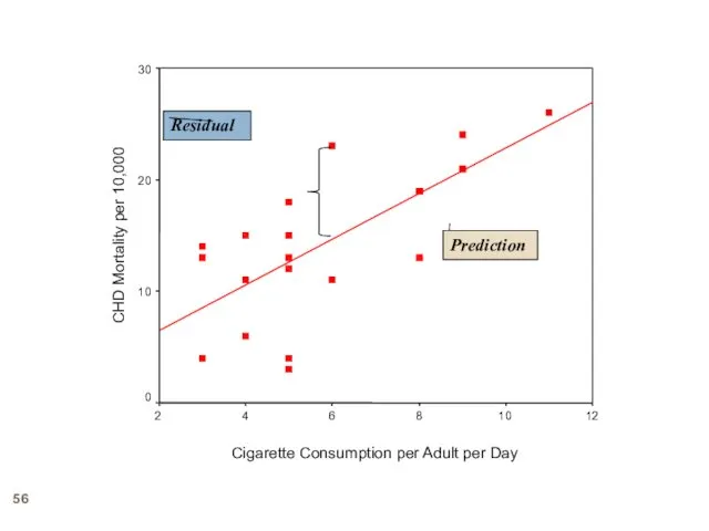
- 56. Cigarette Consumption per Adult per Day 12 10 8 6 4 2 CHD Mortality per 10,000
- 57. Residuals When we predict Ŷ for a given X, we will sometimes be in error. Y
- 58. Minimizing Residuals Again, the problem lies with this definition of the mean: So, how do we
- 60. Скачать презентацию
Causation
Causation
Causation
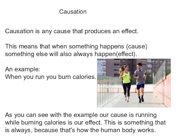
Causation is any cause that produces an effect.
This means that when
Causation
Causation is any cause that produces an effect.
This means that when
Correlation
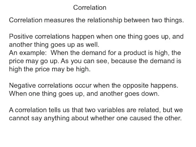
Correlation measures the relationship between two things.
Positive correlations happen when one
Correlation
Correlation measures the relationship between two things.
Positive correlations happen when one
Correlation
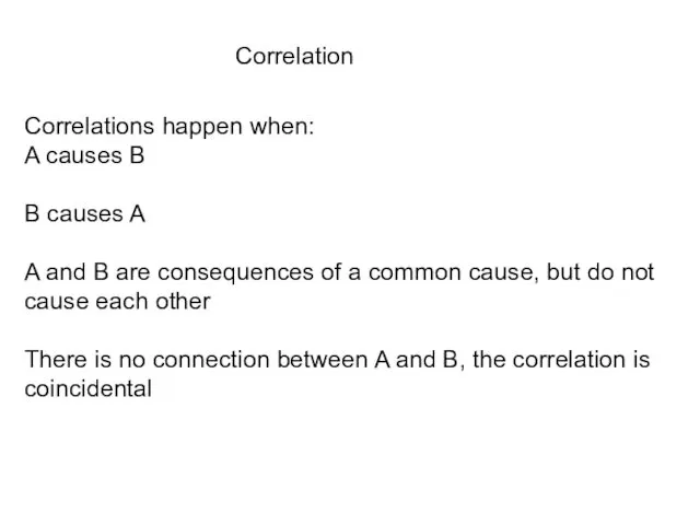
Correlations happen when:
A causes B
B causes A
A and B are consequences
Correlation
Correlations happen when:
A causes B
B causes A
A and B are consequences
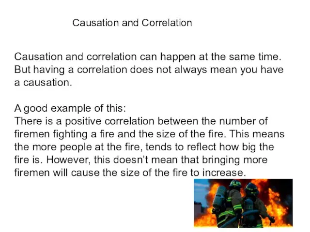
Causation and Correlation
Causation and correlation can happen at the same time.
But
Causation and Correlation
Causation and correlation can happen at the same time.
But
Correlation or Causation?
As people’s happiness level increases, so does their helpfulness.
This
Correlation or Causation?
As people’s happiness level increases, so does their helpfulness.
This
Correlation or Causation?
Dogs pant to cool themselves down.
This would be a
Correlation or Causation?
Dogs pant to cool themselves down.
This would be a
Correlation or Causation?
Among babies, those who are held more tend to
Correlation or Causation?
Among babies, those who are held more tend to
Let's think of our own
Correlation:
Causation:
Let's think of our own
Correlation:
Causation:
Quick Review
Causation is any cause that produces an effect.
Correlation measure the
Quick Review
Causation is any cause that produces an effect.
Correlation measure the
Correlation
Correlation
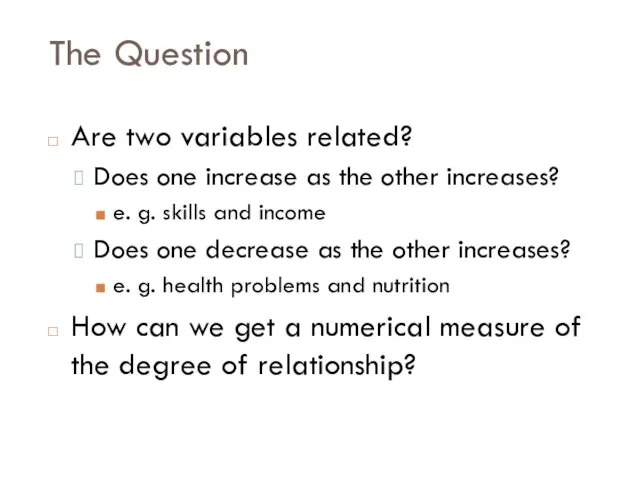
The Question
Are two variables related?
Does one increase as the other increases?
e.
The Question
Are two variables related?
Does one increase as the other increases?
e.
Scatterplots
Graphically depicts the relationship between two variables in two dimensional space.
Scatterplots
Graphically depicts the relationship between two variables in two dimensional space.
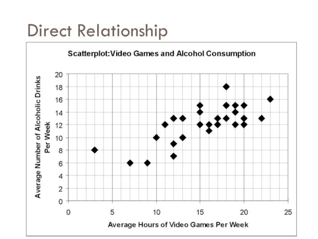
Direct Relationship
Direct Relationship
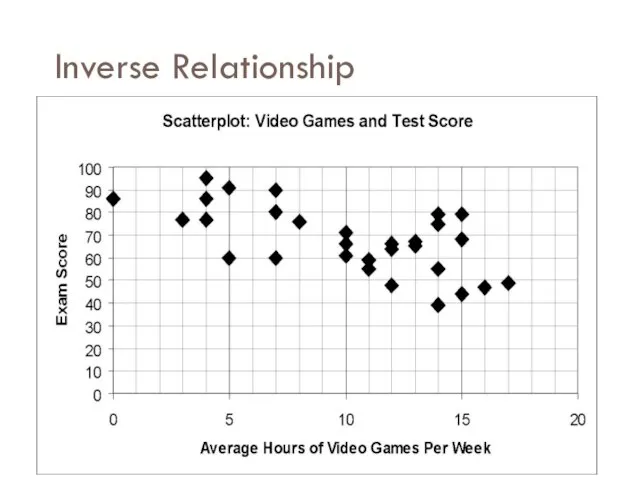
Inverse Relationship
Inverse Relationship
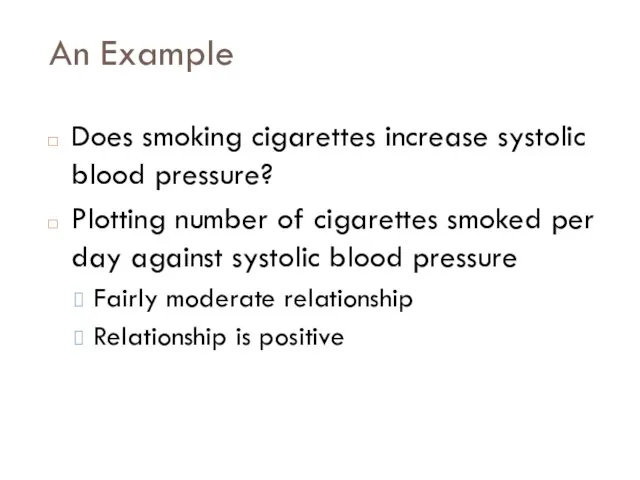
An Example
Does smoking cigarettes increase systolic blood pressure?
Plotting number of cigarettes
An Example
Does smoking cigarettes increase systolic blood pressure?
Plotting number of cigarettes
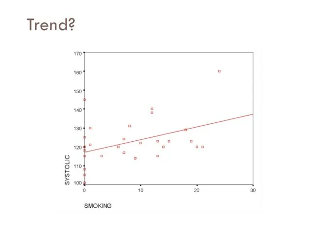
Trend?
Trend?
Smoking and BP
Note relationship is moderate, but real.
Why do we care
Smoking and BP
Note relationship is moderate, but real.
Why do we care
Heart Disease and Cigarettes
Data on heart disease and cigarette smoking in
Heart Disease and Cigarettes
Data on heart disease and cigarette smoking in
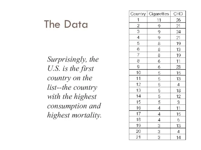
The Data
Surprisingly, the U.S. is the first country on the list--the
The Data
Surprisingly, the U.S. is the first country on the list--the
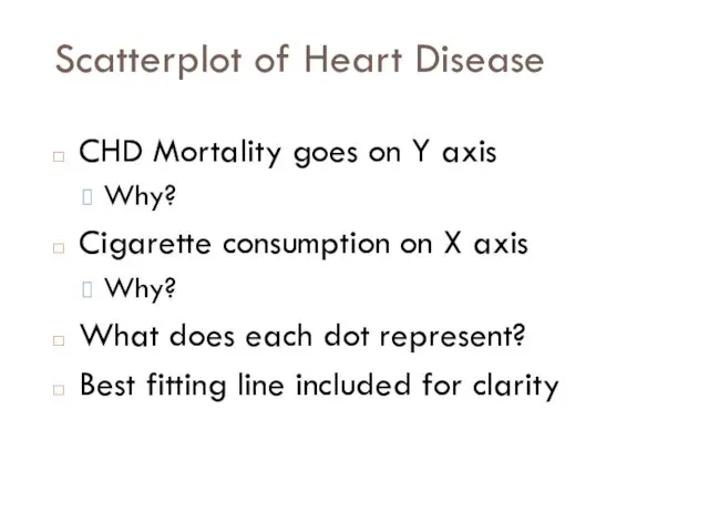
Scatterplot of Heart Disease
CHD Mortality goes on Y axis
Why?
Cigarette consumption on
Scatterplot of Heart Disease
CHD Mortality goes on Y axis
Why?
Cigarette consumption on
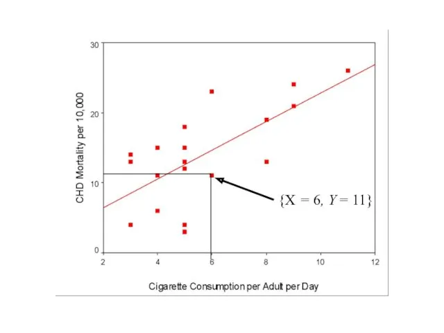
{X = 6, Y = 11}
{X = 6, Y = 11}
What Does the Scatterplot Show?
As smoking increases, so does coronary heart
What Does the Scatterplot Show?
As smoking increases, so does coronary heart
Correlation
Co-relation
The relationship between two variables
Measured with a correlation coefficient
Most popularly seen
Correlation
Co-relation
The relationship between two variables
Measured with a correlation coefficient
Most popularly seen

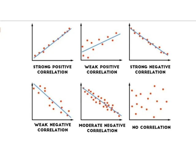
Types of Correlation
Positive correlation
High values of X tend to be associated
Types of Correlation
Positive correlation
High values of X tend to be associated
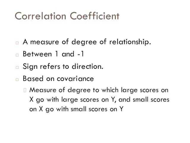
Correlation Coefficient
A measure of degree of relationship.
Between 1 and -1
Sign refers
Correlation Coefficient
A measure of degree of relationship.
Between 1 and -1
Sign refers
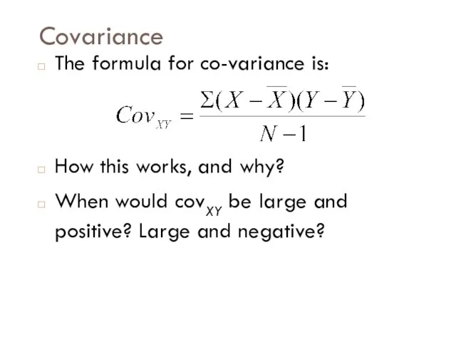
Covariance
The formula for co-variance is:
How this works, and why?
When would covXY
Covariance
The formula for co-variance is:
How this works, and why?
When would covXY
Example
Example
Example
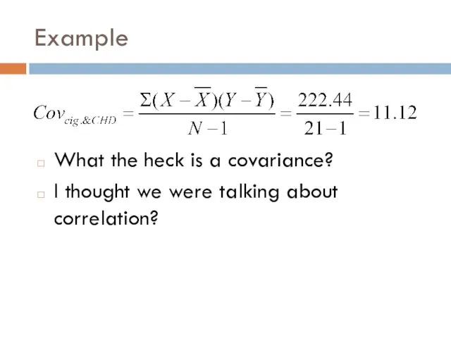
What the heck is a covariance?
I thought we were talking
Example
What the heck is a covariance?
I thought we were talking
Correlation Coefficient
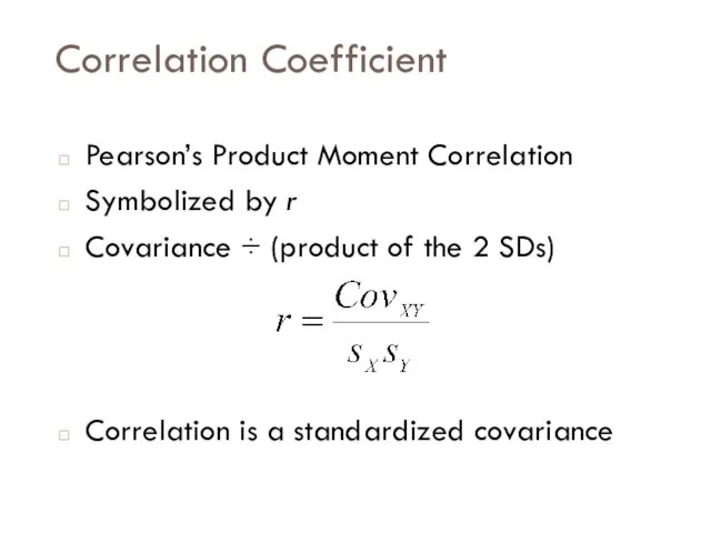
Pearson’s Product Moment Correlation
Symbolized by r
Covariance ÷ (product of the
Correlation Coefficient
Pearson’s Product Moment Correlation
Symbolized by r
Covariance ÷ (product of the
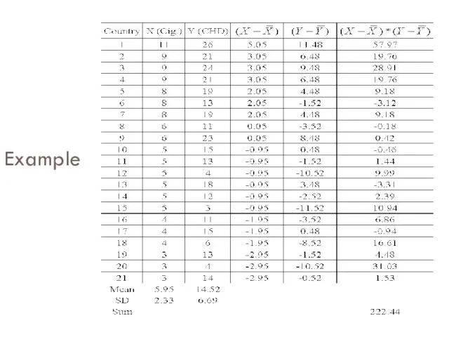
Calculation for Example
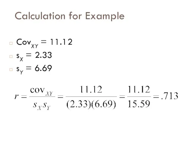
CovXY = 11.12
sX = 2.33
sY = 6.69
Calculation for Example
CovXY = 11.12
sX = 2.33
sY = 6.69
Example
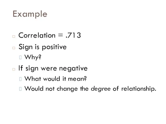
Correlation = .713
Sign is positive
Why?
If sign were negative
What would it mean?
Would
Example
Correlation = .713
Sign is positive
Why?
If sign were negative
What would it mean?
Would
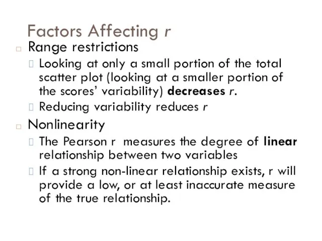
Factors Affecting r
Range restrictions
Looking at only a small portion of the
Factors Affecting r
Range restrictions
Looking at only a small portion of the
Factors Affecting r
Outliers
Overestimate Correlation
Underestimate Correlation
Factors Affecting r
Outliers
Overestimate Correlation
Underestimate Correlation
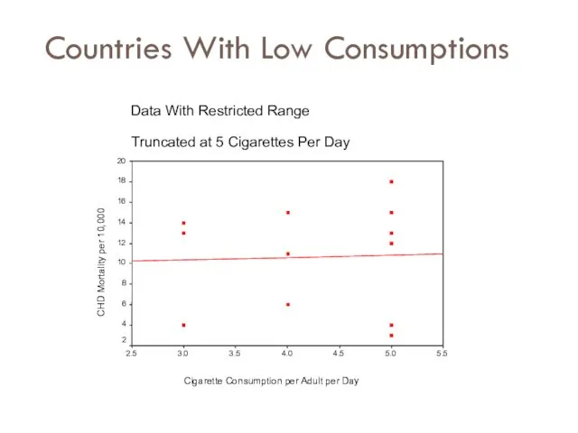
Countries With Low Consumptions
Countries With Low Consumptions

Outliers
Outliers
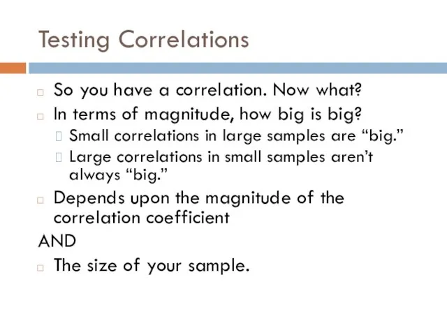
Testing Correlations
So you have a correlation. Now what?
In terms of magnitude,
Testing Correlations
So you have a correlation. Now what?
In terms of magnitude,
Regression
Regression
„Regression” refers to the process of fitting a simple line to
„Regression” refers to the process of fitting a simple line to
What is regression?
How do we predict one variable from another?
How does
What is regression?
How do we predict one variable from another?
How does
Linear Regression
A technique we use to predict the most likely score
Linear Regression
A technique we use to predict the most likely score

Linear Regression: Parts
Y - the variables you are predicting
i.e. dependent variable
X
Linear Regression: Parts
Y - the variables you are predicting
i.e. dependent variable
X
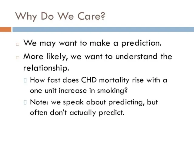
Why Do We Care?
We may want to make a prediction.
More likely,
Why Do We Care?
We may want to make a prediction.
More likely,
An Example
Cigarettes and CHD Mortality again
Data repeated on next slide
We want
An Example
Cigarettes and CHD Mortality again
Data repeated on next slide
We want
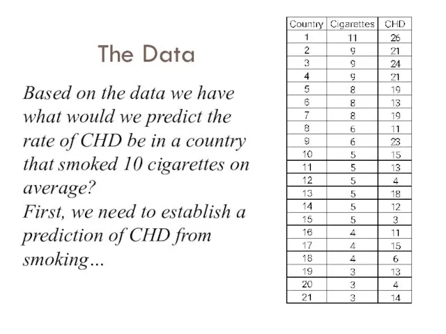
The Data
Based on the data we have what would we predict
The Data
Based on the data we have what would we predict
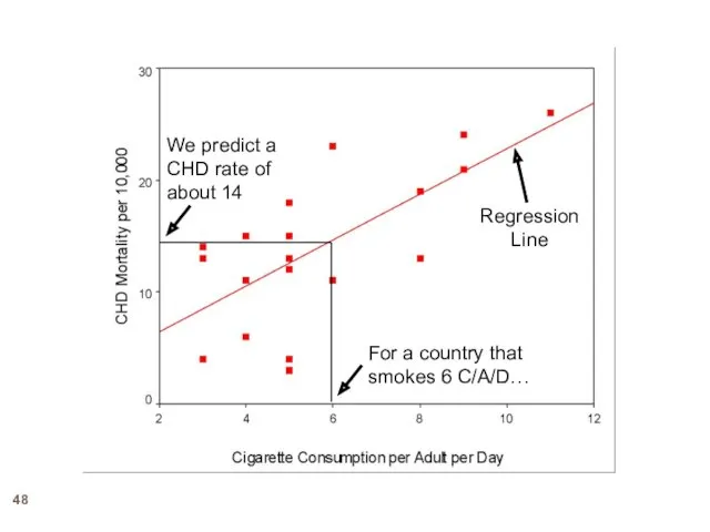
For a country that smokes 6 C/A/D…
We predict a CHD rate
For a country that smokes 6 C/A/D…
We predict a CHD rate
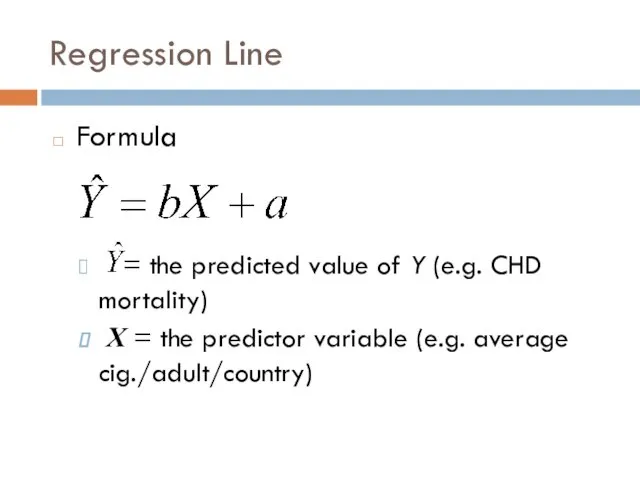
Regression Line
Formula
= the predicted value of Y (e.g. CHD mortality)
X
Regression Line
Formula
= the predicted value of Y (e.g. CHD mortality)
X
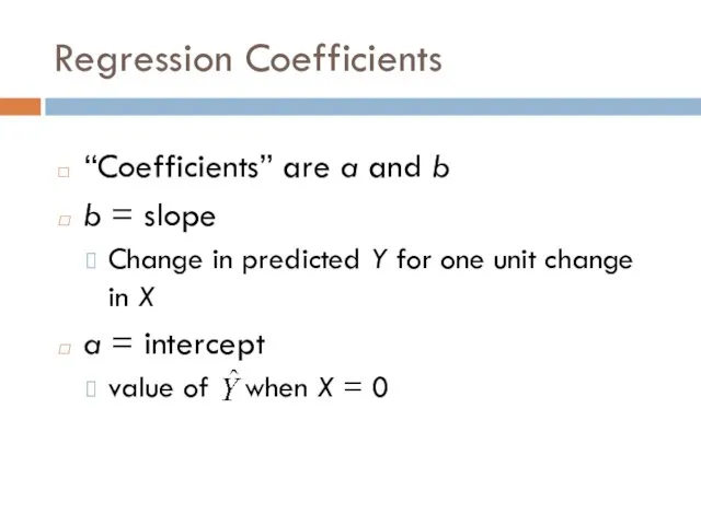
Regression Coefficients
“Coefficients” are a and b
b = slope
Change in predicted
Regression Coefficients
“Coefficients” are a and b
b = slope
Change in predicted
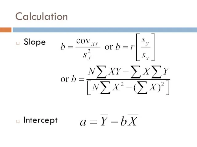
Calculation
Slope
Intercept
Calculation
Slope
Intercept
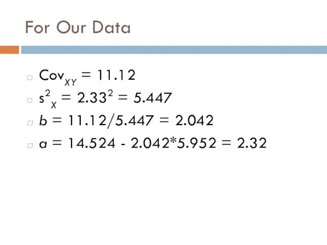
For Our Data
CovXY = 11.12
s2X = 2.332 = 5.447
b = 11.12/5.447
For Our Data
CovXY = 11.12
s2X = 2.332 = 5.447
b = 11.12/5.447
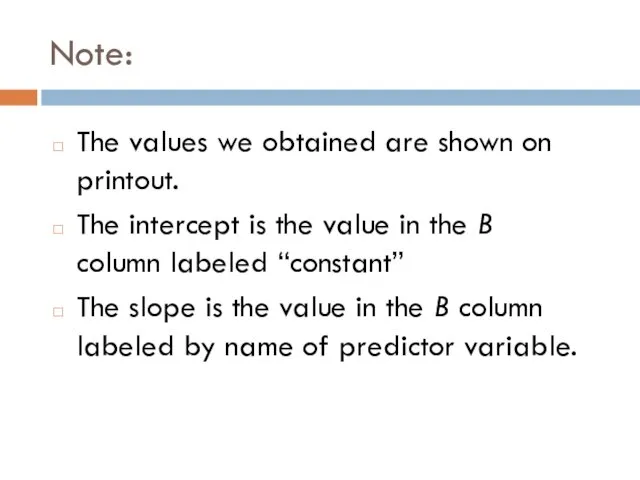
Note:
The values we obtained are shown on printout.
The intercept is the
Note:
The values we obtained are shown on printout.
The intercept is the
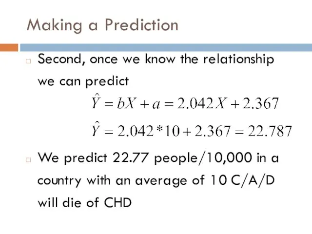
Making a Prediction
Second, once we know the relationship we can predict
We
Making a Prediction
Second, once we know the relationship we can predict
We
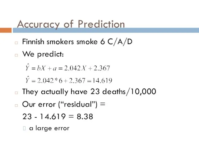
Accuracy of Prediction
Finnish smokers smoke 6 C/A/D
We predict:
They actually have 23
Accuracy of Prediction
Finnish smokers smoke 6 C/A/D
We predict:
They actually have 23
Cigarette Consumption per Adult per Day
12
10
8
6
4
2
CHD Mortality per 10,000
30
20
10
0
Residual
Prediction
Cigarette Consumption per Adult per Day
12
10
8
6
4
2
CHD Mortality per 10,000
30
20
10
0
Residual
Prediction
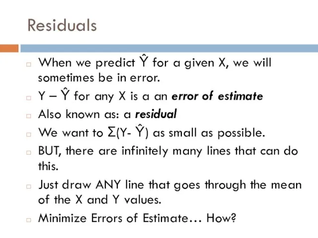
Residuals
When we predict Ŷ for a given X, we will sometimes
Residuals
When we predict Ŷ for a given X, we will sometimes
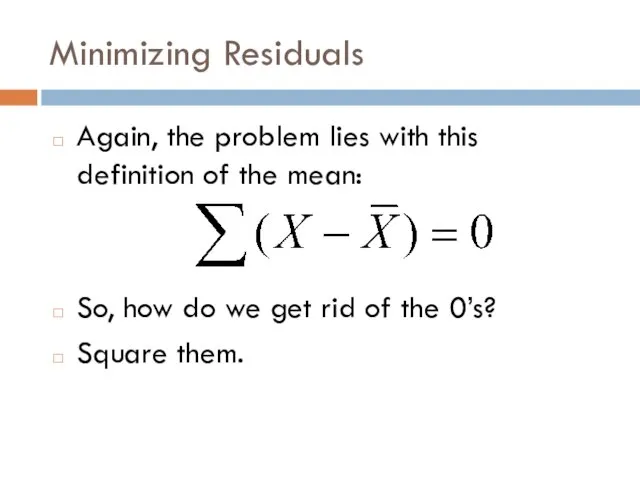
Minimizing Residuals
Again, the problem lies with this definition of the mean:
So,
Minimizing Residuals
Again, the problem lies with this definition of the mean:
So,
 Правило сложения и вычитания обыкновенных дробей с разными знаменателями
 Презентация к уроку математики во 2 классе Умножение и деление на 3. Третья часть числа
 Деление двузначного числа на двузначное способом подбора. (3 класс)
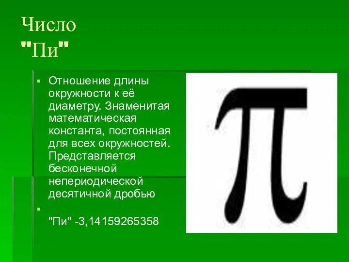 Число Пи
 Сочетательное свойство
 Метод координат при решении геометрических задач
 Нахождение площади фигуры на клетчатой бумаге. Применение формул известных площадей
 Теорема о трех перпендикулярах. Решение задач
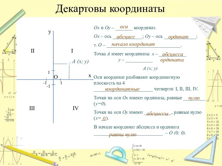 Декартовы координаты
 Обобщение и систематизация знаний по теме Углы и многоугольники
 Состав чисел от 10 до 19
 Решение задач на проценты
 Формула полной вероятности
 Логикалық операциялар (дизъюнкция, конъюнкция, инверсия)
 Транспортир. Измерение углов
 Криві другого порядку
 Арифметичні дії з іменованими числами математика
 Процент от числа
 Параллельные и перпендикулярные прямые. Демонстрационный материал. 6 класс
 Букеты цветов
 Математическое моделирование. Значимость коэффициентов регрессии
 Золотое сечение
 Задания, которые предлагаются детям на подготовительном этапе к изучению нумерации цифр первого десятка
 Число и цифра 10
 Стереометрия. Аксиомы стереометрии
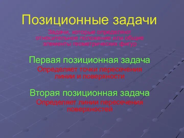 Позиционные задачи
 Примеры комбинаторных задач
 Вектора. Пространства. Скалярное, векторное и смешанное произведение векторов