- Evolution strategies

Содержание
- 2. ES quick overview Developed: Germany in the 1970’s Early names: I. Rechenberg, H.-P. Schwefel Typically applied
- 3. ES technical summary tableau / 30
- 4. Introductory example Task: minimimise f : Rn ? R Algorithm: “two-membered ES” using Vectors from Rn
- 5. Introductory example: pseudocde Set t = 0 Create initial point xt = 〈 x1t,…,xnt 〉 REPEAT
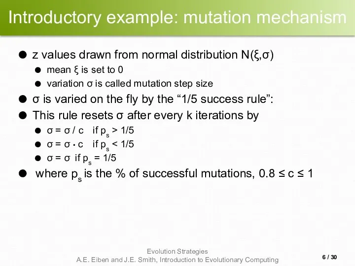
- 6. Introductory example: mutation mechanism z values drawn from normal distribution N(ξ,σ) mean ξ is set to
- 7. Illustration of normal distribution / 30
- 8. Another historical example: the jet nozzle experiment / 30
- 9. The famous jet nozzle experiment (movie) / 30
- 10. Representation Chromosomes consist of three parts: Object variables: x1,…,xn Strategy parameters: Mutation step sizes: σ1,…,σnσ Rotation
- 11. Mutation Main mechanism: changing value by adding random noise drawn from normal distribution x’i = xi
- 12. Mutate σ first Net mutation effect: 〈 x, σ 〉 ? 〈 x’, σ’ 〉 Order
- 13. Mutation case 1: Uncorrelated mutation with one σ Chromosomes: 〈 x1,…,xn, σ 〉 σ’ = σ
- 14. Mutants with equal likelihood Circle: mutants having the same chance to be created / 30
- 15. Mutation case 2: Uncorrelated mutation with n σ’s Chromosomes: 〈 x1,…,xn, σ1,…, σn 〉 σ’i =
- 16. Mutants with equal likelihood Ellipse: mutants having the same chance to be created / 30
- 17. Mutation case 3: Correlated mutations Chromosomes: 〈 x1,…,xn, σ1,…, σn ,α1,…, αk 〉 where k =
- 18. Correlated mutations cont’d The mutation mechanism is then: σ’i = σi • exp(τ’ • N(0,1) +
- 19. Mutants with equal likelihood Ellipse: mutants having the same chance to be created / 30
- 20. Recombination Creates one child Acts per variable / position by either Averaging parental values, or Selecting
- 21. Names of recombinations / 30
- 22. Parent selection Parents are selected by uniform random distribution whenever an operator needs one/some Thus: ES
- 23. Survivor selection Applied after creating λ children from the μ parents by mutation and recombination Deterministically
- 24. Survivor selection cont’d (μ+λ)-selection is an elitist strategy (μ,λ)-selection can “forget” Often (μ,λ)-selection is preferred for:
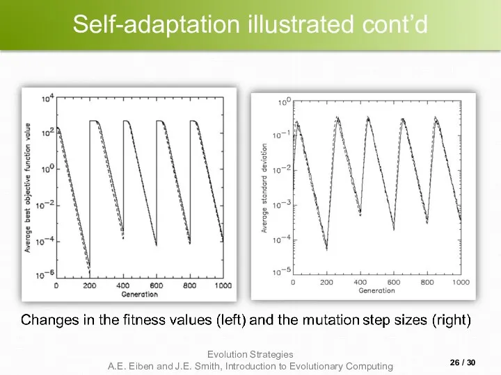
- 25. Self-adaptation illustrated Given a dynamically changing fitness landscape (optimum location shifted every 200 generations) Self-adaptive ES
- 26. Self-adaptation illustrated cont’d / 30
- 27. Prerequisites for self-adaptation μ > 1 to carry different strategies λ > μ to generate offspring
- 28. Example application: the cherry brandy experiment Task: to create a colour mix yielding a target colour
- 29. Example application: cherry brandy experiment cont’d Fitness: students effectively making the mix and comparing it with
- 31. Скачать презентацию
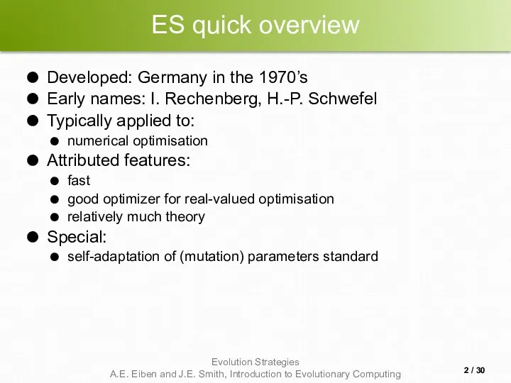
ES quick overview
Developed: Germany in the 1970’s
Early names: I. Rechenberg, H.-P.
ES quick overview
Developed: Germany in the 1970’s
Early names: I. Rechenberg, H.-P.
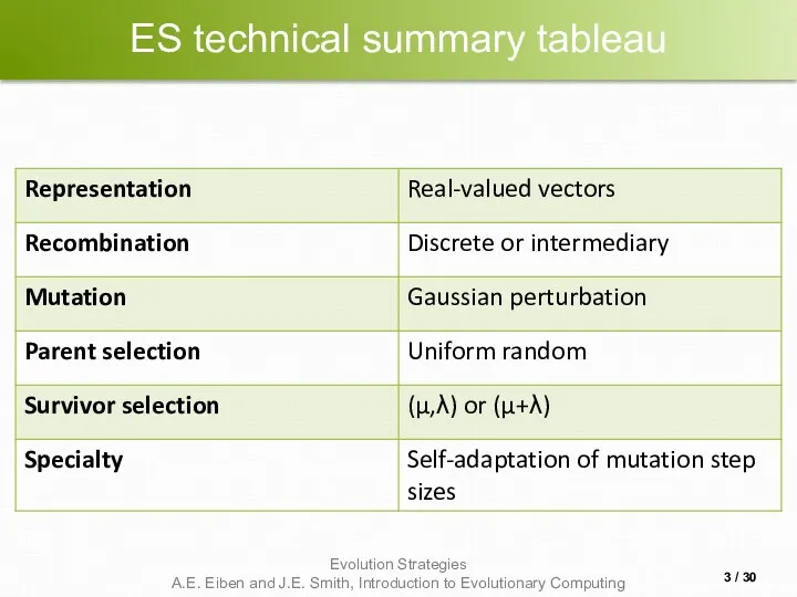
ES technical summary tableau
/ 30
ES technical summary tableau
/ 30
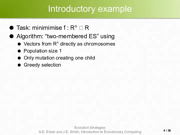
Introductory example
Task: minimimise f : Rn ? R
Algorithm: “two-membered ES” using
Introductory example
Task: minimimise f : Rn ? R
Algorithm: “two-membered ES” using
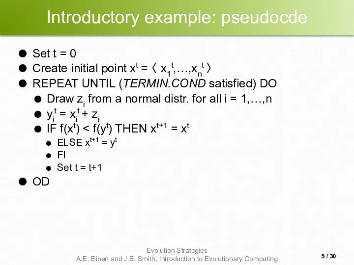
Introductory example: pseudocde
Set t = 0
Create initial point xt = 〈
Introductory example: pseudocde
Set t = 0
Create initial point xt = 〈
Introductory example: mutation mechanism
z values drawn from normal distribution N(ξ,σ)
mean
Introductory example: mutation mechanism
z values drawn from normal distribution N(ξ,σ)
mean
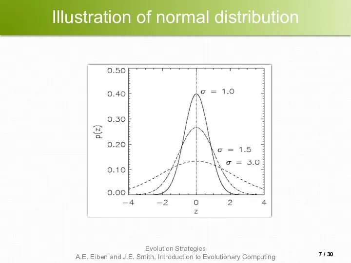
Illustration of normal distribution
/ 30
Illustration of normal distribution
/ 30
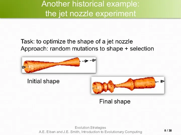
Another historical example:
the jet nozzle experiment
/ 30
Another historical example:
the jet nozzle experiment
/ 30
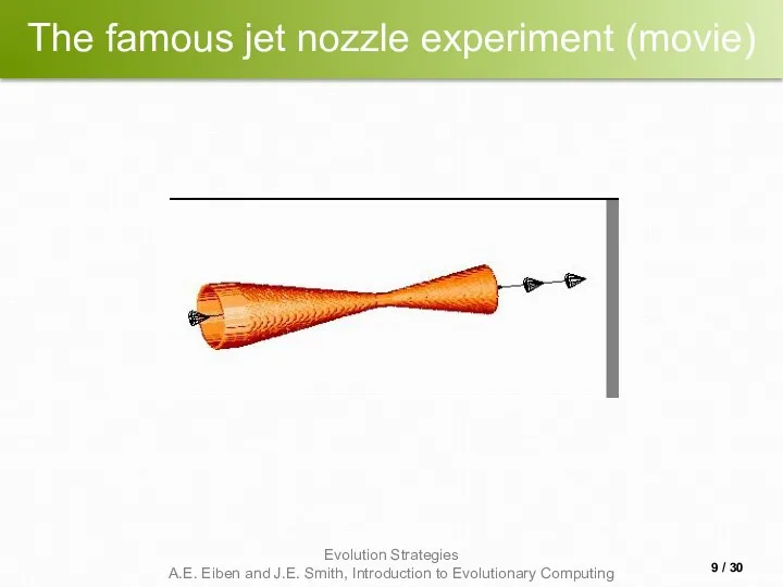
The famous jet nozzle experiment (movie)
/ 30
The famous jet nozzle experiment (movie)
/ 30
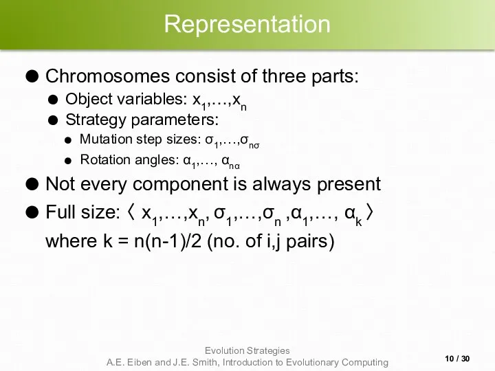
Representation
Chromosomes consist of three parts:
Object variables: x1,…,xn
Strategy parameters:
Mutation step sizes: σ1,…,σnσ
Rotation
Representation
Chromosomes consist of three parts:
Object variables: x1,…,xn
Strategy parameters:
Mutation step sizes: σ1,…,σnσ
Rotation
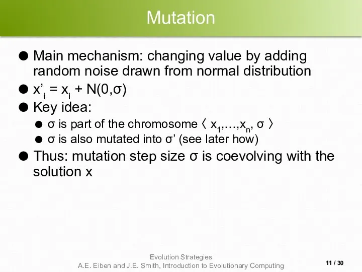
Mutation
Main mechanism: changing value by adding random noise drawn from normal
Mutation
Main mechanism: changing value by adding random noise drawn from normal
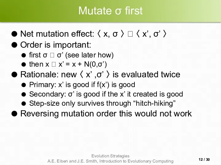
Mutate σ first
Net mutation effect: 〈 x, σ 〉 ? 〈
Mutate σ first
Net mutation effect: 〈 x, σ 〉 ? 〈
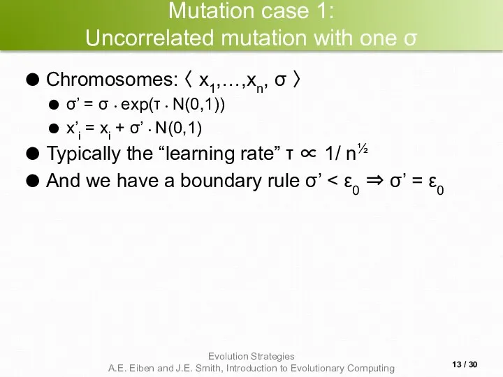
Mutation case 1:
Uncorrelated mutation with one σ
Chromosomes: 〈 x1,…,xn, σ 〉
Mutation case 1:
Uncorrelated mutation with one σ
Chromosomes: 〈 x1,…,xn, σ 〉
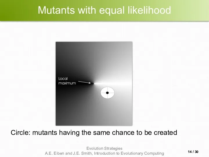
Mutants with equal likelihood
Circle: mutants having the same chance to be
Mutants with equal likelihood
Circle: mutants having the same chance to be
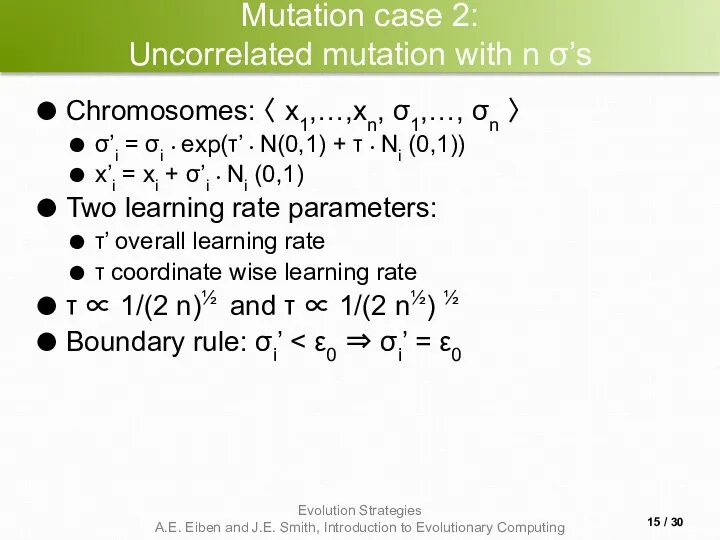
Mutation case 2:
Uncorrelated mutation with n σ’s
Chromosomes: 〈 x1,…,xn, σ1,…, σn
Mutation case 2:
Uncorrelated mutation with n σ’s
Chromosomes: 〈 x1,…,xn, σ1,…, σn
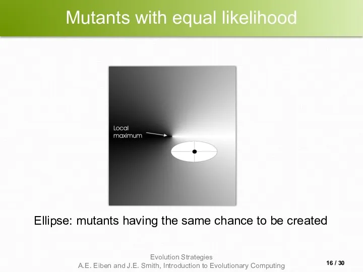
Mutants with equal likelihood
Ellipse: mutants having the same chance to be
Mutants with equal likelihood
Ellipse: mutants having the same chance to be
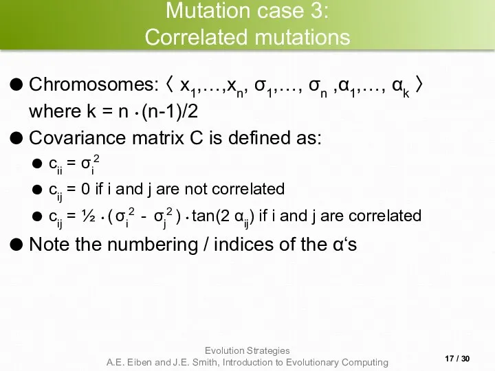
Mutation case 3:
Correlated mutations
Chromosomes: 〈 x1,…,xn, σ1,…, σn ,α1,…, αk
Mutation case 3:
Correlated mutations
Chromosomes: 〈 x1,…,xn, σ1,…, σn ,α1,…, αk
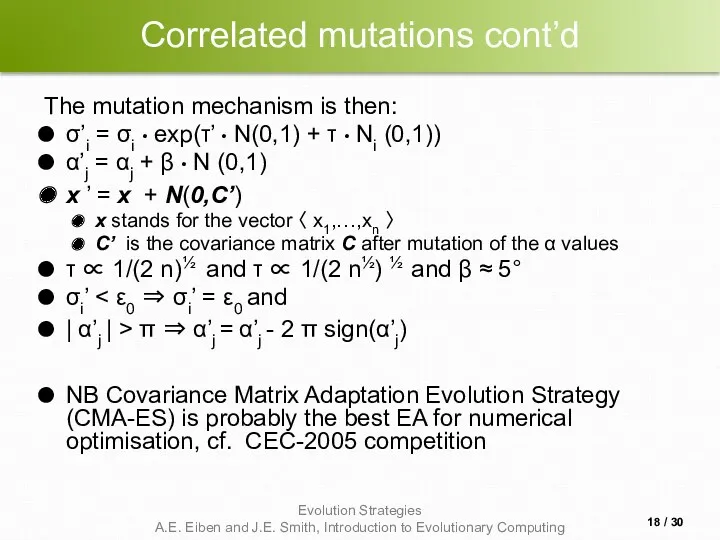
Correlated mutations cont’d
The mutation mechanism is then:
σ’i = σi • exp(τ’
Correlated mutations cont’d
The mutation mechanism is then:
σ’i = σi • exp(τ’
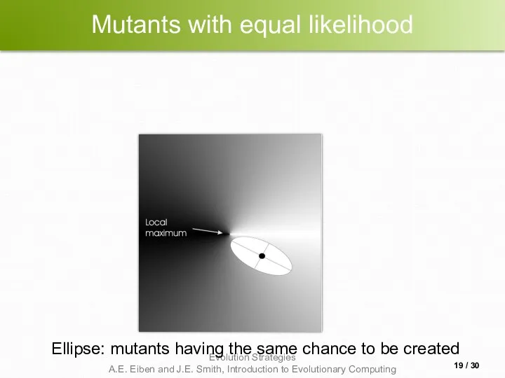
Mutants with equal likelihood
Ellipse: mutants having the same chance to be
Mutants with equal likelihood
Ellipse: mutants having the same chance to be
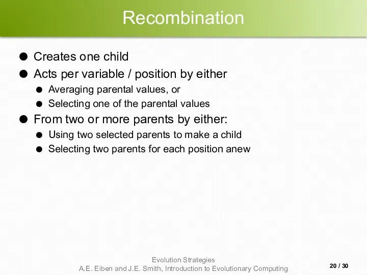
Recombination
Creates one child
Acts per variable / position by either
Averaging parental values,
Recombination
Creates one child
Acts per variable / position by either
Averaging parental values,
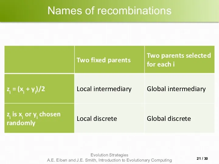
Names of recombinations
/ 30
Names of recombinations
/ 30
Parent selection
Parents are selected by uniform random distribution whenever an operator
Parent selection
Parents are selected by uniform random distribution whenever an operator
Survivor selection
Applied after creating λ children from the μ parents by
Survivor selection
Applied after creating λ children from the μ parents by
Survivor selection cont’d
(μ+λ)-selection is an elitist strategy
(μ,λ)-selection can “forget”
Often (μ,λ)-selection is
Survivor selection cont’d
(μ+λ)-selection is an elitist strategy
(μ,λ)-selection can “forget”
Often (μ,λ)-selection is
Self-adaptation illustrated
Given a dynamically changing fitness landscape (optimum location shifted every
Self-adaptation illustrated
Given a dynamically changing fitness landscape (optimum location shifted every
Self-adaptation illustrated cont’d
/ 30
Self-adaptation illustrated cont’d
/ 30
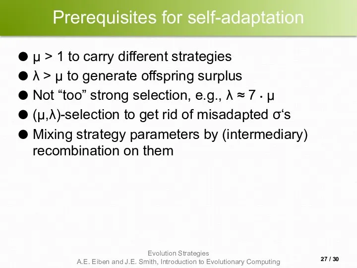
Prerequisites for self-adaptation
μ > 1 to carry different strategies
λ >
Prerequisites for self-adaptation
μ > 1 to carry different strategies
λ >

Example application:
the cherry brandy experiment
Task: to create a colour mix
Example application:
the cherry brandy experiment
Task: to create a colour mix
Example application:
cherry brandy experiment cont’d
Fitness: students effectively making the mix
Example application:
cherry brandy experiment cont’d
Fitness: students effectively making the mix
 Платоновы тела
 Математические сказки
 Понятие движения
 Первые представления о решении рациональных уравнений
 Уравнение прямой
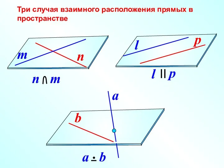 Параллельность прямой и плоскости
 Факторный анализ
 Метапредметные результаты реализации военной составляющей при обучении математике
 Прямая линия в пространстве. Взаимное расположение прямой и плоскости
 Площадь треугольника
 Предел числовой последовательности
 Решение неравенств второй степени с одной переменной
 Решение квадратных уравнений. Формулы корней квадратных уравнений. 8 класс
 Признаки параллельности прямых. Задачи на готовых чертежах
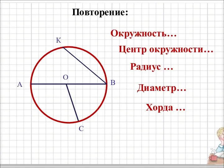 Окружность. Центр окружности
 Сложение и вычитание чисел
 Объект и предмет метрологии
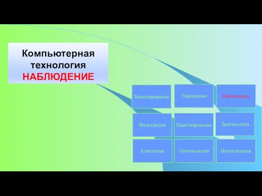 Компьютерная технология. Наблюдение
 Линейные дискретные системы. Структура звеньев второго порядка
 Понятие движения
 Урок математики Название и запись трехзначных чисел Диск
 Математическое моделирование
 Нахождение гамильтонова контура минимальной длины. Задача коммивояжера
 Одночлен. Арифметические операции над одночленами
 Визначник другого та третього порядків. Алгебраїчні доповнення
 Учимся определять время по часам
 Решение задач с помощью дробно – рациональных уравнений
 Непрерывность функции. Непрерывность функции в точке