- Modeling non-stationary variables

Содержание
- 2. Lecture Objectives Revisit the concept of non-stationary (unit root) process and its implications for analysis and
- 3. Outline Stationary and non-stationary variables Testing for unit roots Cointegration Testing for cointegration
- 4. Introduction Macro-econometric Forecasting and Analysis Many economic (macro/financial) variables exhibit trending behavior e.g., real GDP, real
- 5. Key Macro Series Appear to have trends Macro-econometric Forecasting and Analysis
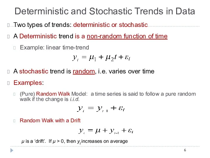
- 6. Deterministic and Stochastic Trends in Data Two types of trends: deterministic or stochastic A Deterministic trend
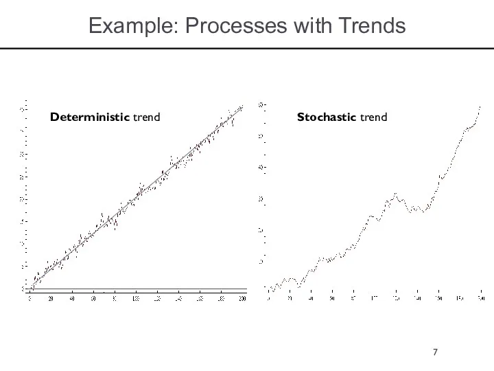
- 7. Example: Processes with Trends Deterministic trend Stochastic trend
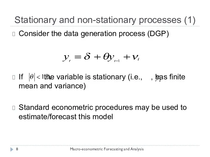
- 8. Stationary and non-stationary processes (1) Macro-econometric Forecasting and Analysis Consider the data generation process (DGP) If
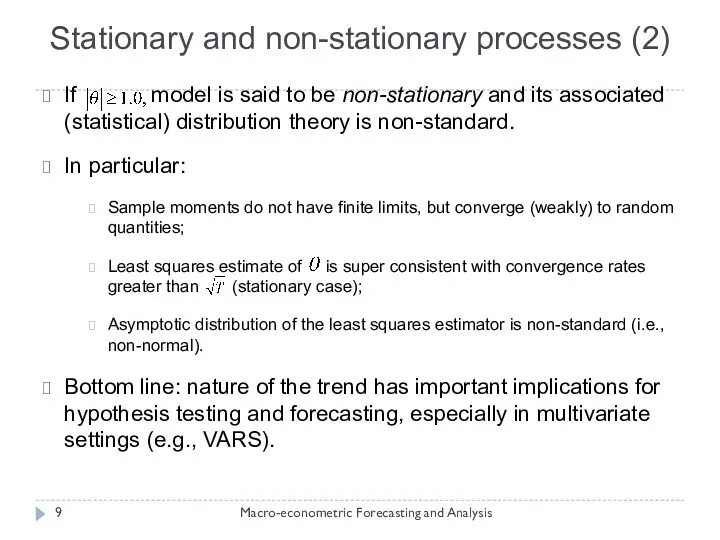
- 9. Macro-econometric Forecasting and Analysis If model is said to be non-stationary and its associated (statistical) distribution
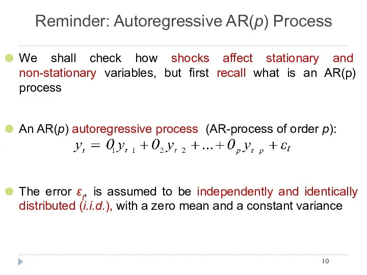
- 10. Reminder: Autoregressive AR(p) Process We shall check how shocks affect stationary and non-stationary variables, but first
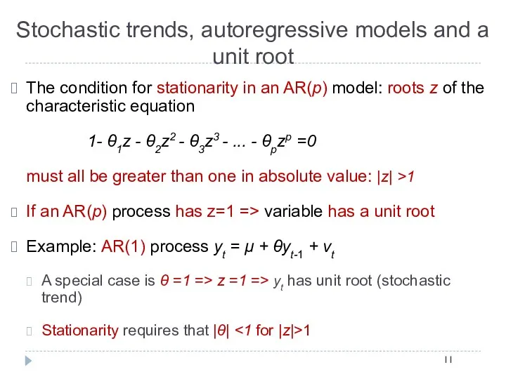
- 11. Stochastic trends, autoregressive models and a unit root The condition for stationarity in an AR(p) model:
- 12. Consider a simple AR(1): yt = θyt-1 + νt, where θ takes any value for now
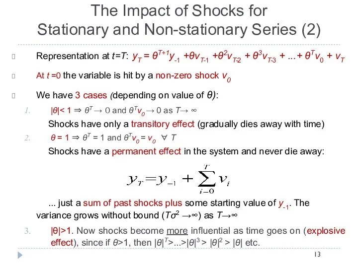
- 13. The Impact of Shocks for Stationary and Non-stationary Series (2) Representation at t=T: yT = θT+1y-1
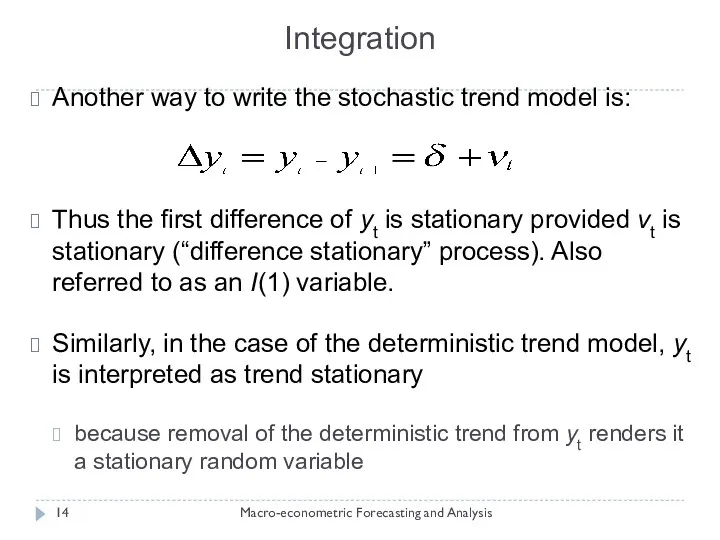
- 14. Integration Macro-econometric Forecasting and Analysis Another way to write the stochastic trend model is: Thus the
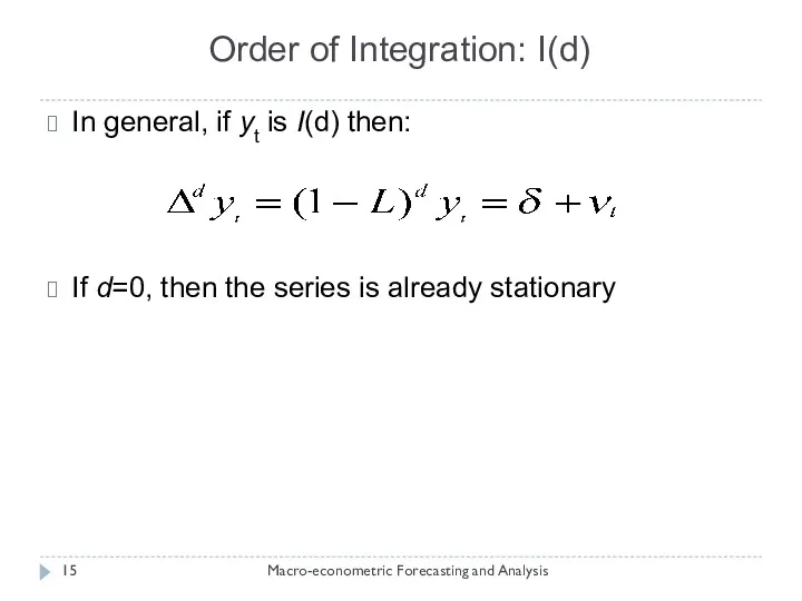
- 15. Order of Integration: I(d) Macro-econometric Forecasting and Analysis In general, if yt is I(d) then: If
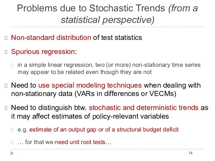
- 16. Problems due to Stochastic Trends (from a statistical perspective) Non-standard distribution of test statistics Spurious regression:
- 17. Figure 5: Distribution of OLS estimator for θ Macro-econometric Forecasting and Analysis
- 18. Testing For Unit Roots Macro-econometric Forecasting and Analysis Previous section suggests that I(1) variables need special
- 19. Testing for Unit Roots: Procedures Dickey Fuller Augmented Dickey Fuller Phillips Perron Kwiatkowski, Phillips, Schmidt and
- 20. Dickey Fuller Test Fuller (1976), Dickey and Fuller (1979) Example: consider a particular case of an
- 21. Dickey-Fuller Test (2) For the purpose of testing we reformulate the regression: Δyt = yt –
- 22. Dickey-Fuller Test (3) Important issue – shall deterministic components be included in the test model for
- 23. DF-Test (3): Deterministic Components are Known Say, we assume yt includes an intercept, but not a
- 24. If deterministic components are not included in the test, when they should be, then the test
- 25. The Augmented Dickey Fuller (ADF) Test The DF-test above is only valid if εt is a
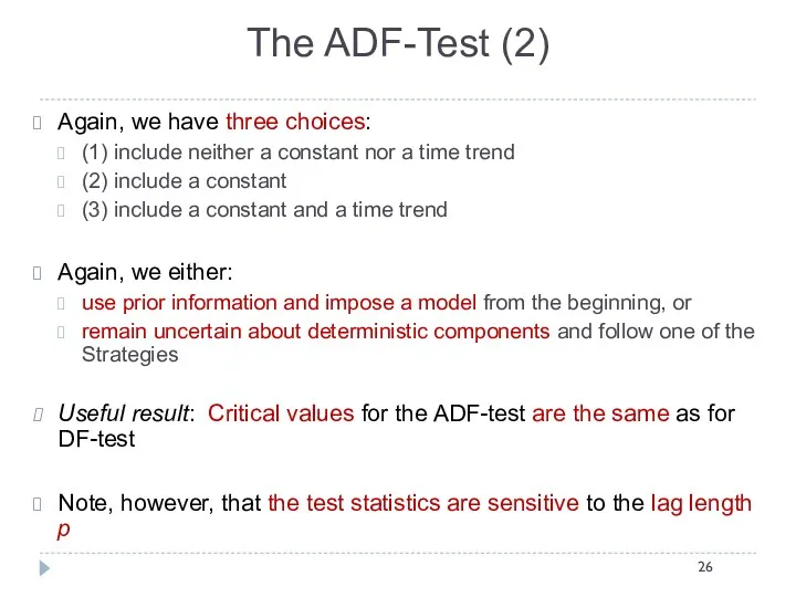
- 26. The ADF-Test (2) Again, we have three choices: (1) include neither a constant nor a time
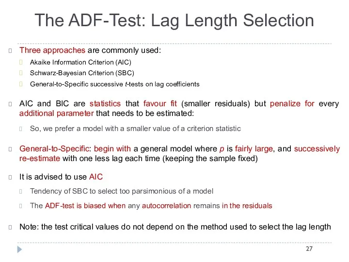
- 27. The ADF-Test: Lag Length Selection Three approaches are commonly used: Akaike Information Criterion (AIC) Schwarz-Bayesian Criterion
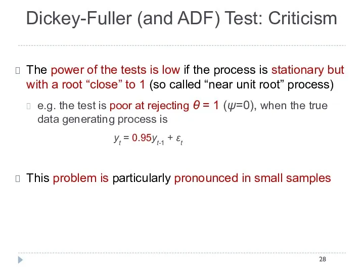
- 28. Dickey-Fuller (and ADF) Test: Criticism The power of the tests is low if the process is
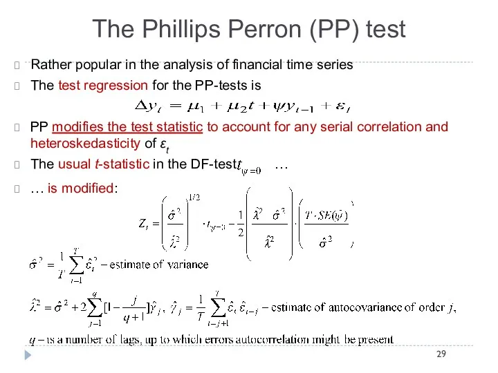
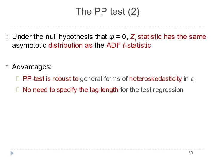
- 29. The Phillips Perron (PP) test Rather popular in the analysis of financial time series The test
- 30. The PP test (2) Under the null hypothesis that ψ = 0, Zt statistic has the
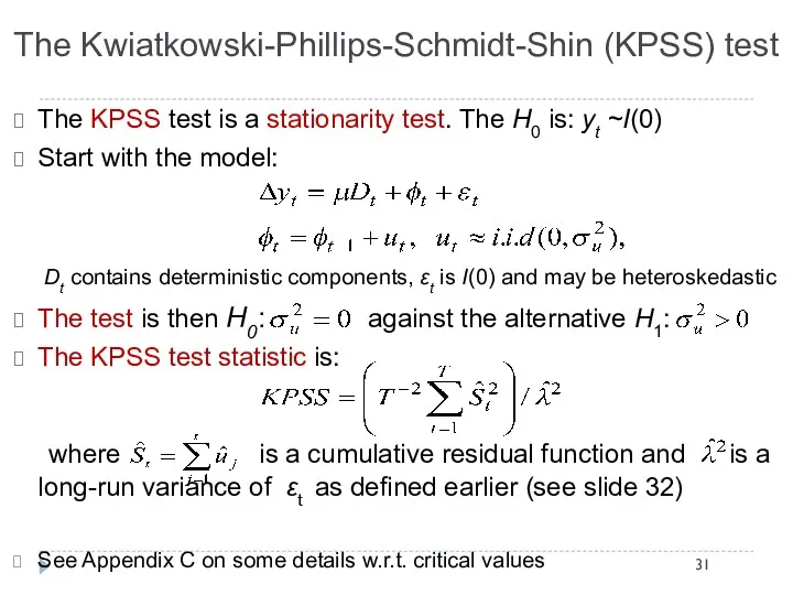
- 31. The Kwiatkowski-Phillips-Schmidt-Shin (KPSS) test The KPSS test is a stationarity test. The H0 is: yt ~I(0)
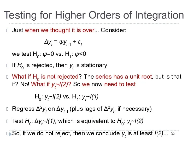
- 32. Testing for Higher Orders of Integration Just when we thought it is over... Consider: Δyt =
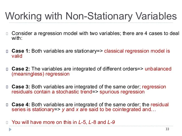
- 33. Working with Non-Stationary Variables Consider a regression model with two variables; there are 4 cases to
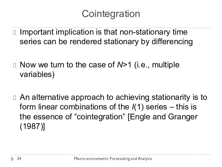
- 34. Cointegration Macro-econometric Forecasting and Analysis Important implication is that non-stationary time series can be rendered stationary
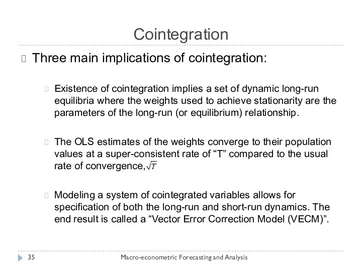
- 35. Cointegration Macro-econometric Forecasting and Analysis Three main implications of cointegration: Existence of cointegration implies a set
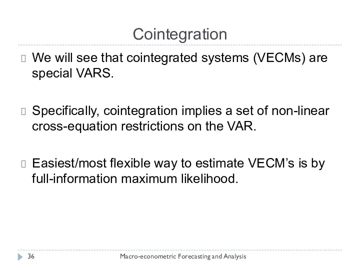
- 36. Cointegration Macro-econometric Forecasting and Analysis We will see that cointegrated systems (VECMs) are special VARS. Specifically,
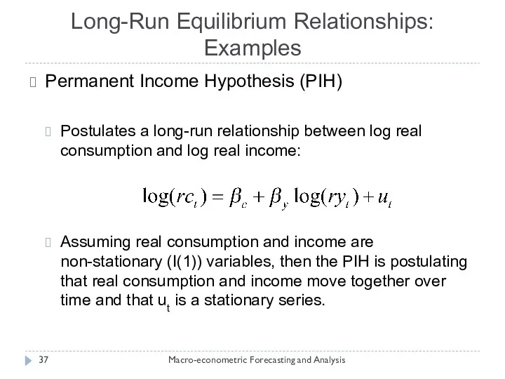
- 37. Long-Run Equilibrium Relationships: Examples Macro-econometric Forecasting and Analysis Permanent Income Hypothesis (PIH) Postulates a long-run relationship
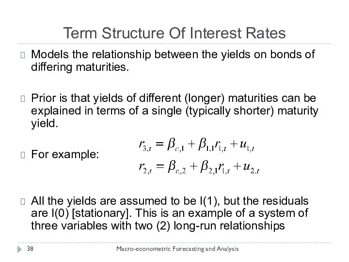
- 38. Term Structure Of Interest Rates Macro-econometric Forecasting and Analysis Models the relationship between the yields on
- 39. VECM Macro-econometric Forecasting and Analysis Cointegration postulates the existence of long-run equilibrium relationships between non-stationary variables
- 40. Bivariate VECMs Macro-econometric Forecasting and Analysis Consider a bivariate model containing two I(1) variables, say Assume
- 41. Phase Diagram: VECM Macro-econometric Forecasting and Analysis
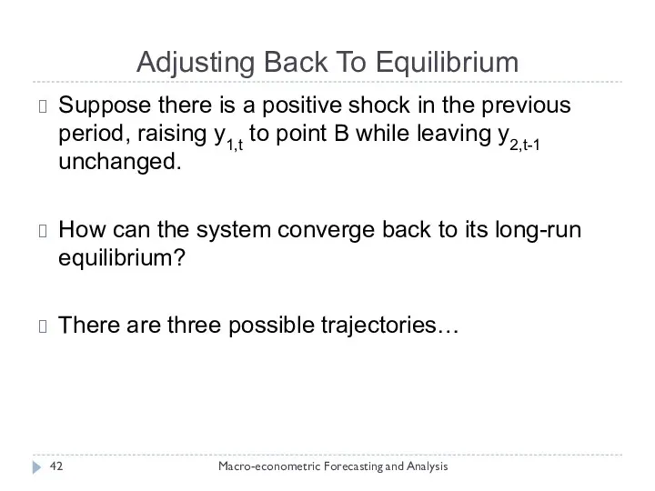
- 42. Adjusting Back To Equilibrium Macro-econometric Forecasting and Analysis Suppose there is a positive shock in the
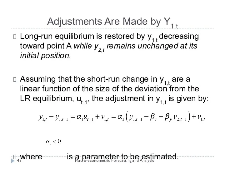
- 43. Adjustments Are Made by Y1,t Macro-econometric Forecasting and Analysis Long-run equilibrium is restored by y1,t decreasing
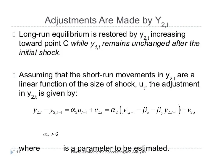
- 44. Adjustments Are Made by Y2,t Macro-econometric Forecasting and Analysis Long-run equilibrium is restored by y2,t increasing
- 45. Adjustments are made by both Y1,t and Y2,t Macro-econometric Forecasting and Analysis The previous two equations
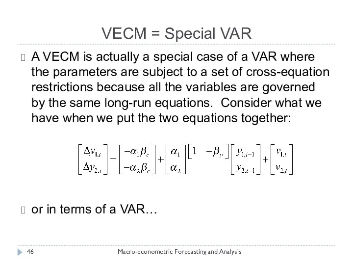
- 46. VECM = Special VAR Macro-econometric Forecasting and Analysis A VECM is actually a special case of
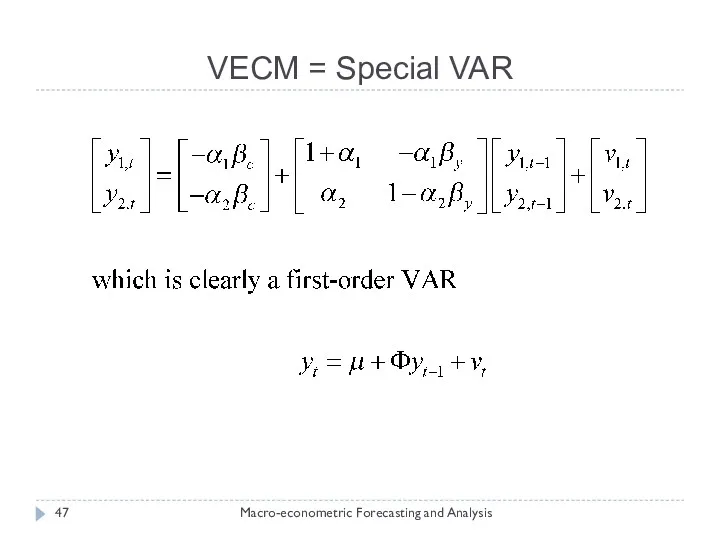
- 47. VECM = Special VAR Macro-econometric Forecasting and Analysis
- 48. VECM = Special VAR Macro-econometric Forecasting and Analysis Obviously, we have a first order VAR with
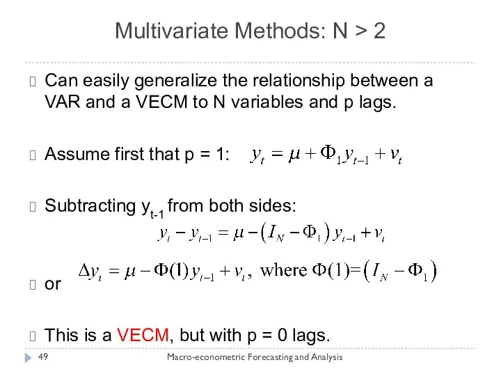
- 49. Multivariate Methods: N > 2 Macro-econometric Forecasting and Analysis Can easily generalize the relationship between a
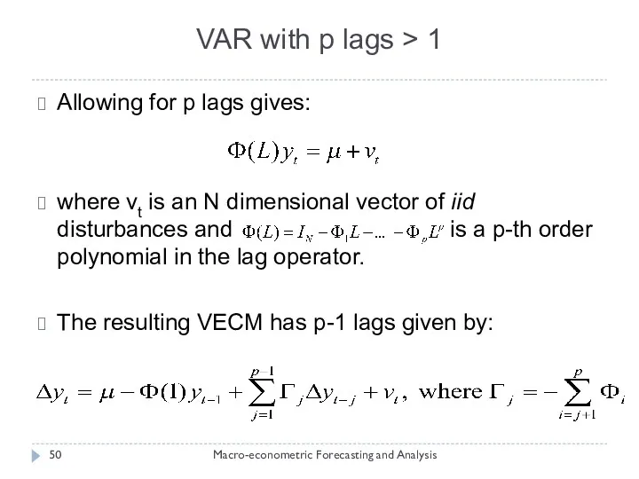
- 50. VAR with p lags > 1 Macro-econometric Forecasting and Analysis Allowing for p lags gives: where
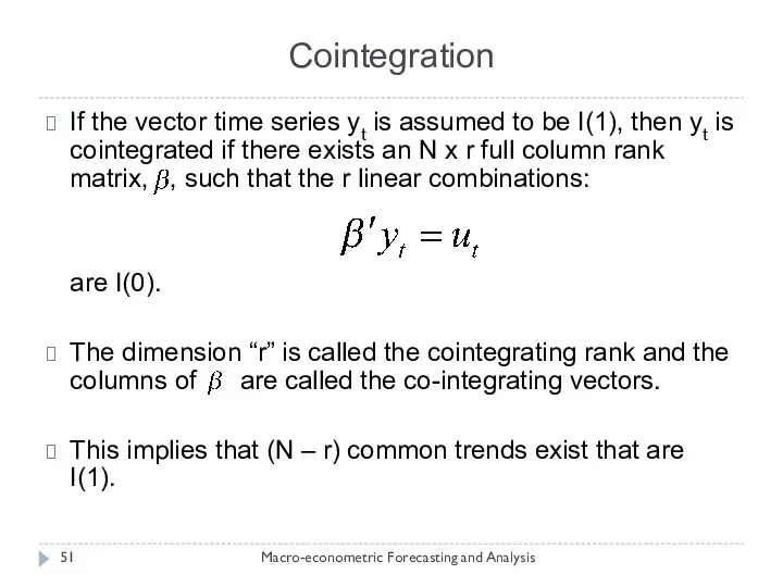
- 51. Cointegration Macro-econometric Forecasting and Analysis If the vector time series yt is assumed to be I(1),
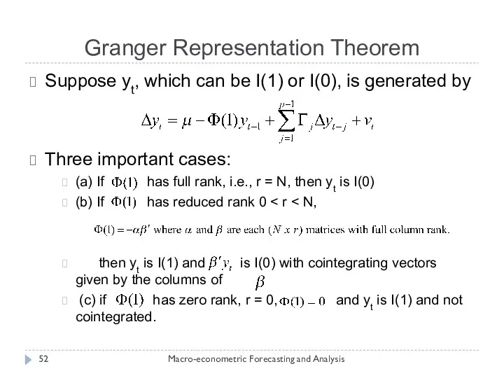
- 52. Granger Representation Theorem Macro-econometric Forecasting and Analysis Suppose yt, which can be I(1) or I(0), is
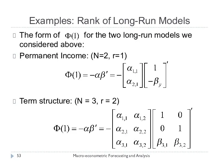
- 53. Examples: Rank of Long-Run Models Macro-econometric Forecasting and Analysis The form of for the two long-run
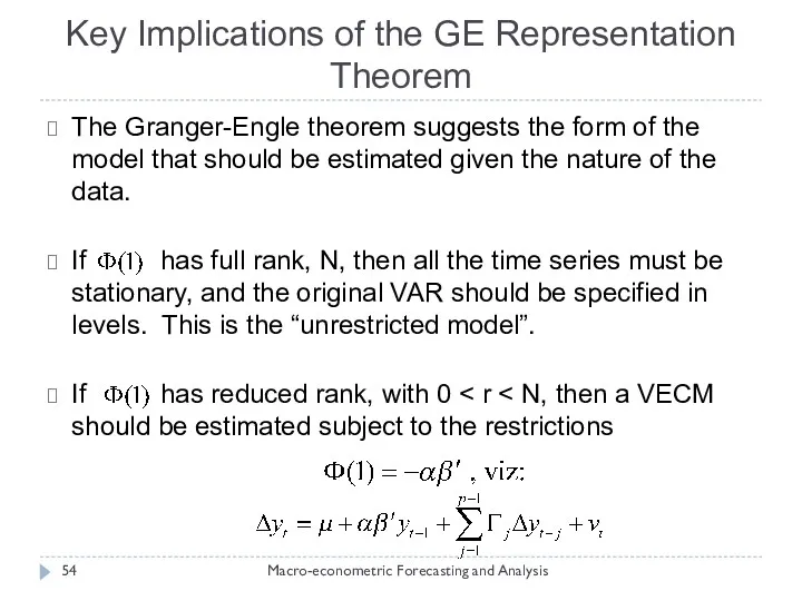
- 54. Key Implications of the GE Representation Theorem Macro-econometric Forecasting and Analysis The Granger-Engle theorem suggests the
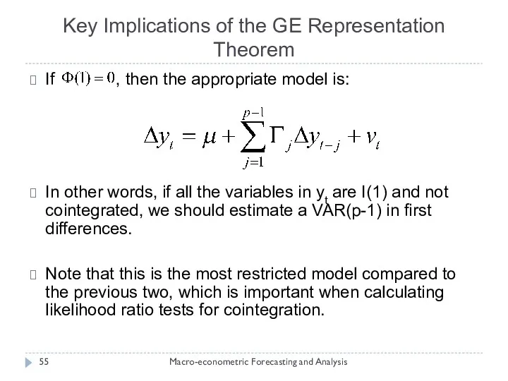
- 55. Key Implications of the GE Representation Theorem Macro-econometric Forecasting and Analysis If , then the appropriate
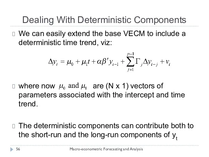
- 56. Dealing With Deterministic Components Macro-econometric Forecasting and Analysis We can easily extend the base VECM to
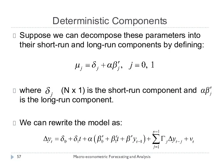
- 57. Deterministic Components Macro-econometric Forecasting and Analysis Suppose we can decompose these parameters into their short-run and
- 58. Deterministic Components Macro-econometric Forecasting and Analysis The term represents the long-run relationship among the variables. The
- 59. Deterministic Components Macro-econometric Forecasting and Analysis The equation contains five important special cases summarized on the
- 60. Alternative Deterministic Structures Macro-econometric Forecasting and Analysis
- 61. Estimating VECM Models Macro-econometric Forecasting and Analysis If you are willing to assume that the error
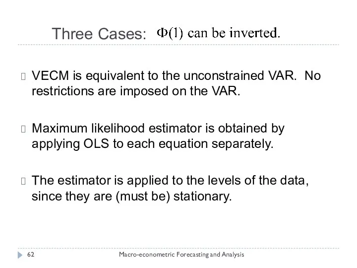
- 62. Three Cases: Macro-econometric Forecasting and Analysis VECM is equivalent to the unconstrained VAR. No restrictions are
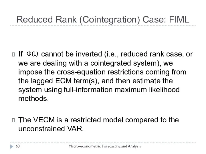
- 63. Reduced Rank (Cointegration) Case: FIML Macro-econometric Forecasting and Analysis If cannot be inverted (i.e., reduced rank
- 64. Reduced Rank Case: Johansen Estimator Macro-econometric Forecasting and Analysis We can also use the Johansen (1988)
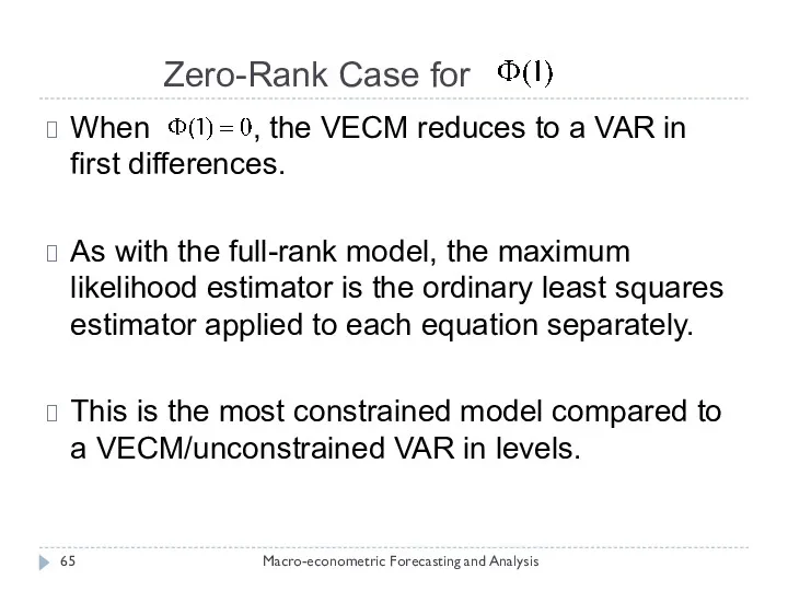
- 65. Zero-Rank Case for Macro-econometric Forecasting and Analysis When , the VECM reduces to a VAR in
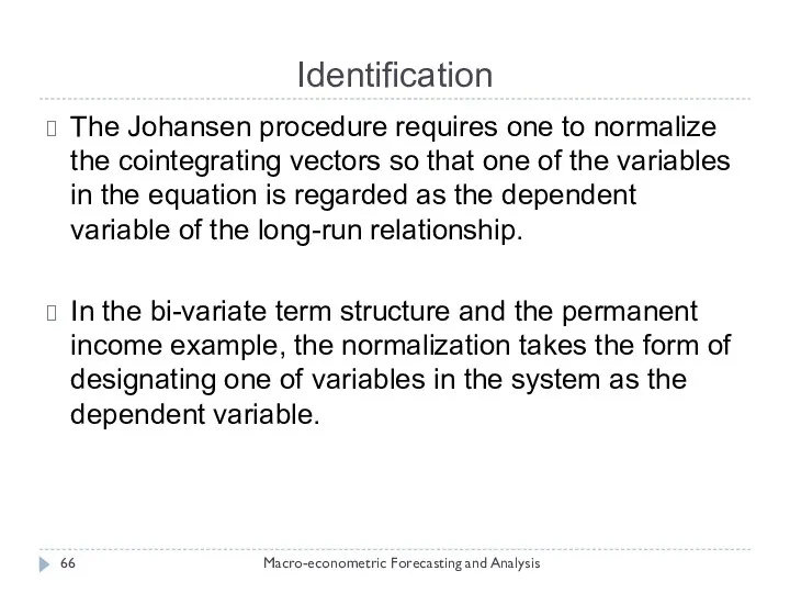
- 66. Identification Macro-econometric Forecasting and Analysis The Johansen procedure requires one to normalize the cointegrating vectors so
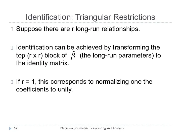
- 67. Identification: Triangular Restrictions Macro-econometric Forecasting and Analysis Suppose there are r long-run relationships. Identification can be
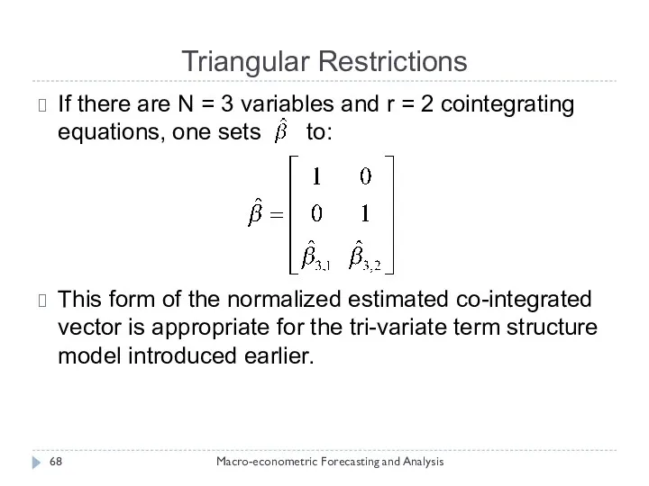
- 68. Triangular Restrictions Macro-econometric Forecasting and Analysis If there are N = 3 variables and r =
- 69. Structural Restrictions Macro-econometric Forecasting and Analysis Traditional identification methods can also be used with VECM’s, including
- 70. Open Economy Model Macro-econometric Forecasting and Analysis Assuming r = 2 long-run equations, the following restrictions
- 71. Cointegration Rank Macro-econometric Forecasting and Analysis So far we have taken the rank of the system
- 72. Cointegration Rank: Likelihood Ratio Test Macro-econometric Forecasting and Analysis Suppose we estimate the model assuming no
- 73. Cointegration Rank: Likelihood Ratio Test Macro-econometric Forecasting and Analysis Using the standard result for the likelihood
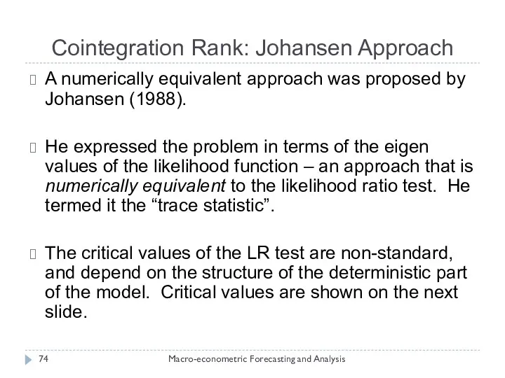
- 74. Cointegration Rank: Johansen Approach Macro-econometric Forecasting and Analysis A numerically equivalent approach was proposed by Johansen
- 75. Critical Values of the Likelihood Ratio Test Macro-econometric Forecasting and Analysis
- 76. Tests on the Cointegrating Vector (Long-Run Parameters) Macro-econometric Forecasting and Analysis Hypothesis tests on the cointegrating
- 77. Exogeneity Macro-econometric Forecasting and Analysis An important feature of a VECM is that all of the
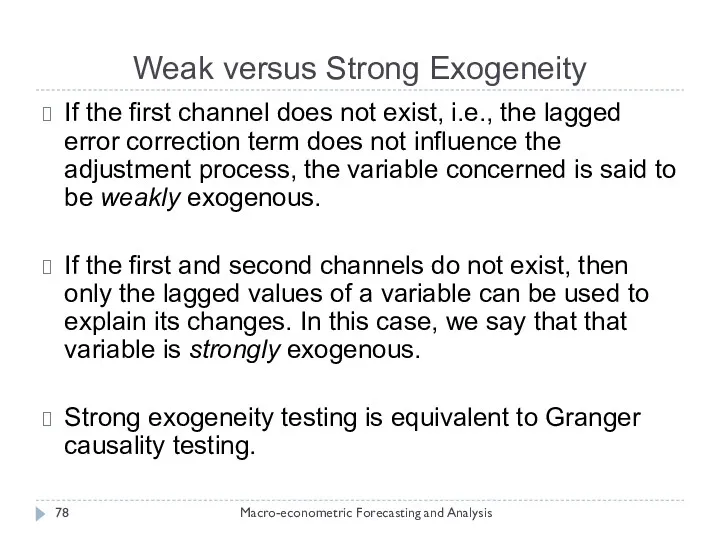
- 78. Weak versus Strong Exogeneity Macro-econometric Forecasting and Analysis If the first channel does not exist, i.e.,
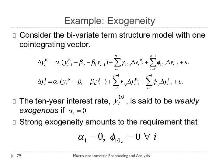
- 79. Example: Exogeneity Macro-econometric Forecasting and Analysis Consider the bi-variate term structure model with one cointegrating vector.
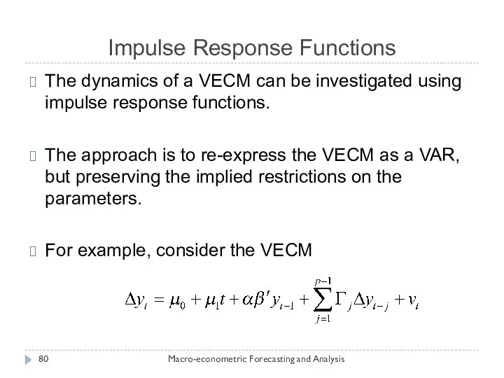
- 80. Impulse Response Functions Macro-econometric Forecasting and Analysis The dynamics of a VECM can be investigated using
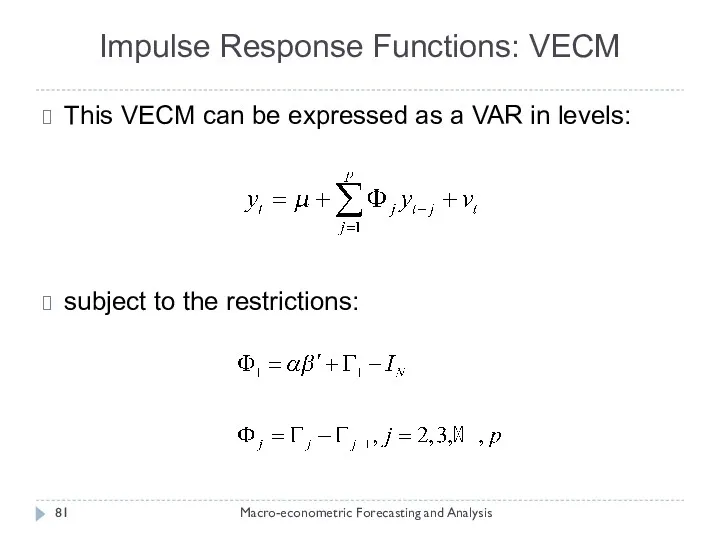
- 81. Impulse Response Functions: VECM Macro-econometric Forecasting and Analysis This VECM can be expressed as a VAR
- 82. Appendices
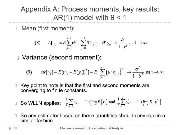
- 83. Appendix A: Process moments, key results: AR(1) model with θ Macro-econometric Forecasting and Analysis Mean (first
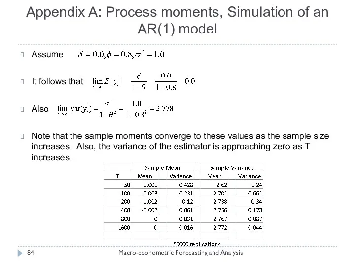
- 84. Appendix A: Process moments, Simulation of an AR(1) model Macro-econometric Forecasting and Analysis Assume It follows
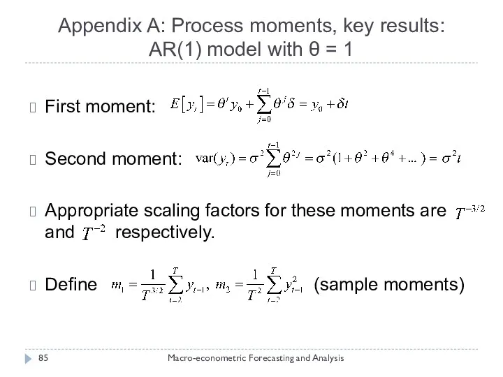
- 85. Appendix A: Process moments, key results: AR(1) model with θ = 1 Macro-econometric Forecasting and Analysis
- 86. Appendix A: Process moments, simulation of an I(1) Process Macro-econometric Forecasting and Analysis Notice that the
- 87. Appendix B: Enders Strategy Test H0: ψ=0 t-ratio test, 5% Crit. value is -3.45 Estimate Δyt
- 88. Enders Strategy was criticized for: triple- and double-testing for unit roots unrealistic outcomes: economic variables unlikely
- 89. Appendix B: Elder and Kennedy Strategy Test H0: ψ=0 t-ratio test, 5% Crit. value is -3.45
- 90. Nonstationary Asymptotics Macro-econometric Forecasting and Analysis
- 92. Скачать презентацию
Lecture Objectives
Revisit the concept of non-stationary (unit root) process and
Lecture Objectives
Revisit the concept of non-stationary (unit root) process and
Outline
Stationary and non-stationary variables
Testing for unit roots
Cointegration
Testing for cointegration
Outline
Stationary and non-stationary variables
Testing for unit roots
Cointegration
Testing for cointegration
Introduction
Macro-econometric Forecasting and Analysis
Many economic (macro/financial) variables exhibit trending behavior
e.g.,
Introduction
Macro-econometric Forecasting and Analysis
Many economic (macro/financial) variables exhibit trending behavior
e.g.,
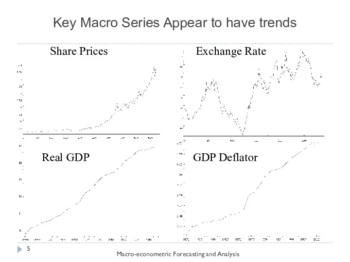
Key Macro Series Appear to have trends
Macro-econometric Forecasting and Analysis
Key Macro Series Appear to have trends
Macro-econometric Forecasting and Analysis
Deterministic and Stochastic Trends in Data
Two types of trends: deterministic or
Deterministic and Stochastic Trends in Data
Two types of trends: deterministic or
Example: Processes with Trends
Deterministic trend
Stochastic trend
Example: Processes with Trends
Deterministic trend
Stochastic trend
Stationary and non-stationary processes (1)
Macro-econometric Forecasting and Analysis
Consider the data generation
Stationary and non-stationary processes (1)
Macro-econometric Forecasting and Analysis
Consider the data generation
Macro-econometric Forecasting and Analysis
If model is said to be non-stationary and
Macro-econometric Forecasting and Analysis
If model is said to be non-stationary and
Reminder: Autoregressive AR(p) Process
We shall check how shocks affect stationary and
Reminder: Autoregressive AR(p) Process
We shall check how shocks affect stationary and
Stochastic trends, autoregressive models and a unit root
The condition for stationarity
Stochastic trends, autoregressive models and a unit root
The condition for stationarity
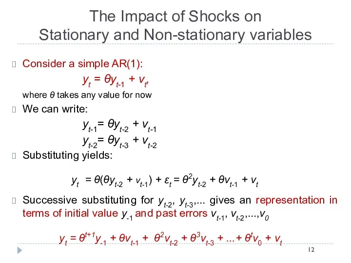
Consider a simple AR(1):
yt = θyt-1 + νt,
where θ takes
Consider a simple AR(1):
yt = θyt-1 + νt,
where θ takes
The Impact of Shocks for
Stationary and Non-stationary Series (2)
Representation at
The Impact of Shocks for
Stationary and Non-stationary Series (2)
Representation at
Integration
Macro-econometric Forecasting and Analysis
Another way to write the stochastic trend model
Integration
Macro-econometric Forecasting and Analysis
Another way to write the stochastic trend model
Order of Integration: I(d)
Macro-econometric Forecasting and Analysis
In general, if yt is
Order of Integration: I(d)
Macro-econometric Forecasting and Analysis
In general, if yt is
Problems due to Stochastic Trends (from a statistical perspective)
Non-standard distribution of
Problems due to Stochastic Trends (from a statistical perspective)
Non-standard distribution of
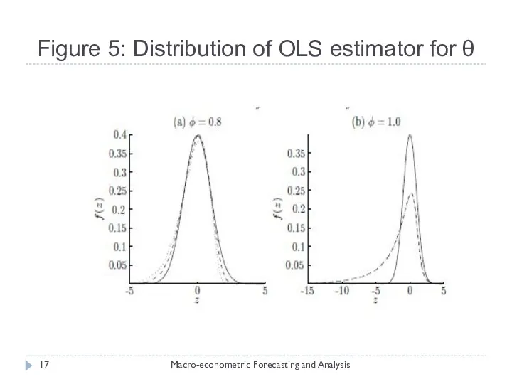
Figure 5: Distribution of OLS estimator for θ
Macro-econometric Forecasting and Analysis
Figure 5: Distribution of OLS estimator for θ
Macro-econometric Forecasting and Analysis
Testing For Unit Roots
Macro-econometric Forecasting and Analysis
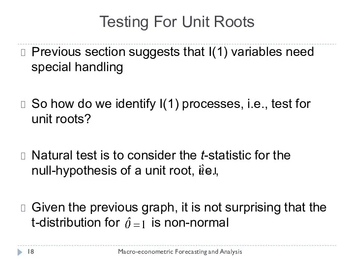
Previous section suggests that I(1)
Testing For Unit Roots
Macro-econometric Forecasting and Analysis
Previous section suggests that I(1)
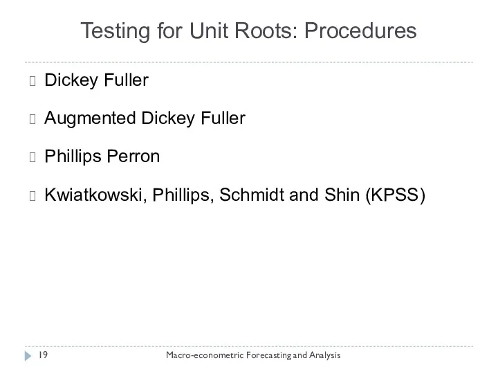
Testing for Unit Roots: Procedures
Dickey Fuller
Augmented Dickey Fuller
Phillips Perron
Kwiatkowski, Phillips, Schmidt
Testing for Unit Roots: Procedures
Dickey Fuller
Augmented Dickey Fuller
Phillips Perron
Kwiatkowski, Phillips, Schmidt
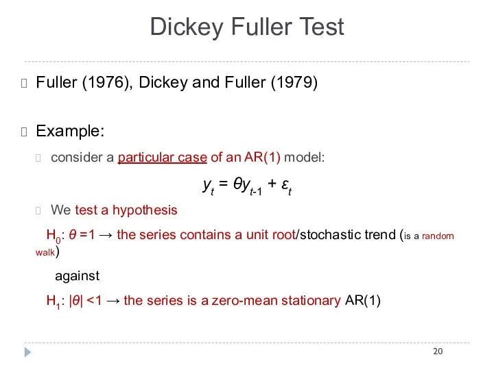
Dickey Fuller Test
Fuller (1976), Dickey and Fuller (1979)
Example:
consider a particular
Dickey Fuller Test
Fuller (1976), Dickey and Fuller (1979)
Example:
consider a particular
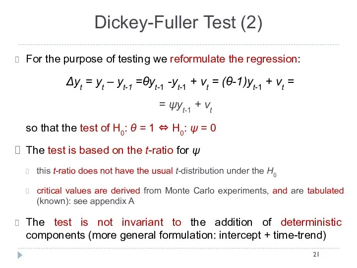
Dickey-Fuller Test (2)
For the purpose of testing we reformulate the regression:
Δyt
Dickey-Fuller Test (2)
For the purpose of testing we reformulate the regression:
Δyt
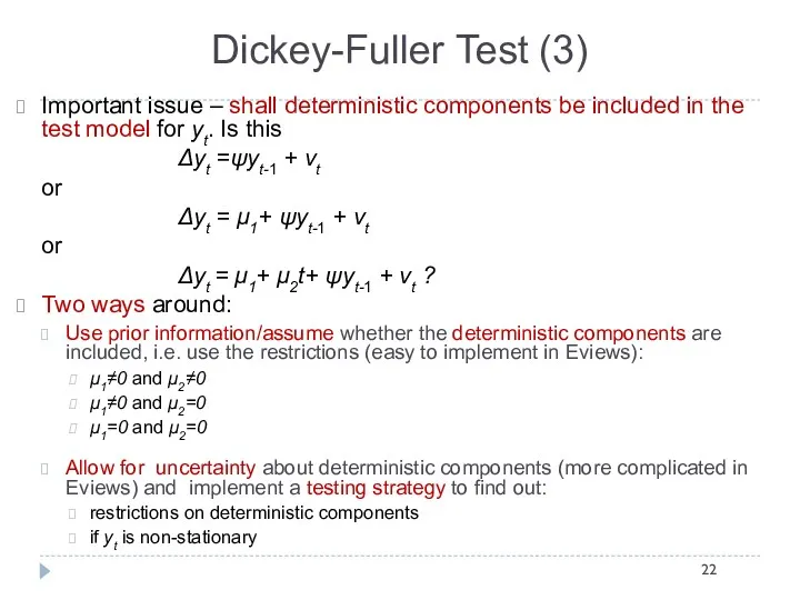
Dickey-Fuller Test (3)
Important issue – shall deterministic components be included in
Dickey-Fuller Test (3)
Important issue – shall deterministic components be included in
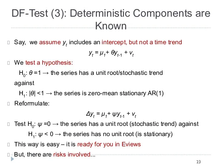
DF-Test (3): Deterministic Components are Known
Say, we assume yt includes an
DF-Test (3): Deterministic Components are Known
Say, we assume yt includes an
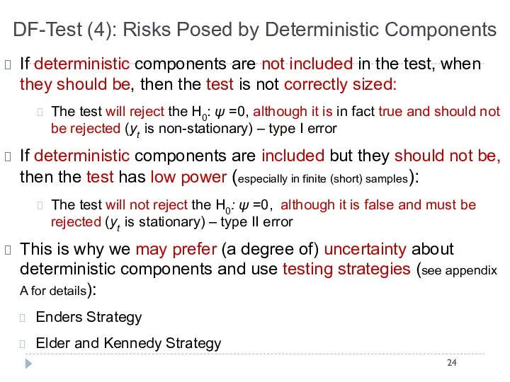
If deterministic components are not included in the test, when they
If deterministic components are not included in the test, when they
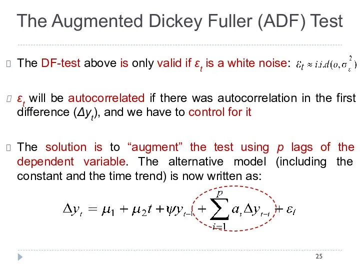
The Augmented Dickey Fuller (ADF) Test
The DF-test above is only valid
The Augmented Dickey Fuller (ADF) Test
The DF-test above is only valid
The ADF-Test (2)
Again, we have three choices:
(1) include neither a constant
The ADF-Test (2)
Again, we have three choices:
(1) include neither a constant
The ADF-Test: Lag Length Selection
Three approaches are commonly used:
Akaike Information
The ADF-Test: Lag Length Selection
Three approaches are commonly used:
Akaike Information
Dickey-Fuller (and ADF) Test: Criticism
The power of the tests is low
Dickey-Fuller (and ADF) Test: Criticism
The power of the tests is low
The Phillips Perron (PP) test
Rather popular in the analysis of financial
The Phillips Perron (PP) test
Rather popular in the analysis of financial
The PP test (2)
Under the null hypothesis that ψ = 0,
The PP test (2)
Under the null hypothesis that ψ = 0,
The Kwiatkowski-Phillips-Schmidt-Shin (KPSS) test
The KPSS test is a stationarity test. The
The Kwiatkowski-Phillips-Schmidt-Shin (KPSS) test
The KPSS test is a stationarity test. The
Testing for Higher Orders of Integration
Just when we thought it is
Testing for Higher Orders of Integration
Just when we thought it is
Working with Non-Stationary Variables
Consider a regression model with two variables; there
Working with Non-Stationary Variables
Consider a regression model with two variables; there
Cointegration
Macro-econometric Forecasting and Analysis
Important implication is that non-stationary time series can
Cointegration
Macro-econometric Forecasting and Analysis
Important implication is that non-stationary time series can
Cointegration
Macro-econometric Forecasting and Analysis
Three main implications of cointegration:
Existence of cointegration implies
Cointegration
Macro-econometric Forecasting and Analysis
Three main implications of cointegration:
Existence of cointegration implies
Cointegration
Macro-econometric Forecasting and Analysis
We will see that cointegrated systems (VECMs) are
Cointegration
Macro-econometric Forecasting and Analysis
We will see that cointegrated systems (VECMs) are
Long-Run Equilibrium Relationships: Examples
Macro-econometric Forecasting and Analysis
Permanent Income Hypothesis (PIH)
Postulates a
Long-Run Equilibrium Relationships: Examples
Macro-econometric Forecasting and Analysis
Permanent Income Hypothesis (PIH)
Postulates a
Term Structure Of Interest Rates
Macro-econometric Forecasting and Analysis
Models the relationship between
Term Structure Of Interest Rates
Macro-econometric Forecasting and Analysis
Models the relationship between
VECM
Macro-econometric Forecasting and Analysis
Cointegration postulates the existence of long-run equilibrium relationships
VECM
Macro-econometric Forecasting and Analysis
Cointegration postulates the existence of long-run equilibrium relationships
Bivariate VECMs
Macro-econometric Forecasting and Analysis
Consider a bivariate model containing two I(1)
Bivariate VECMs
Macro-econometric Forecasting and Analysis
Consider a bivariate model containing two I(1)
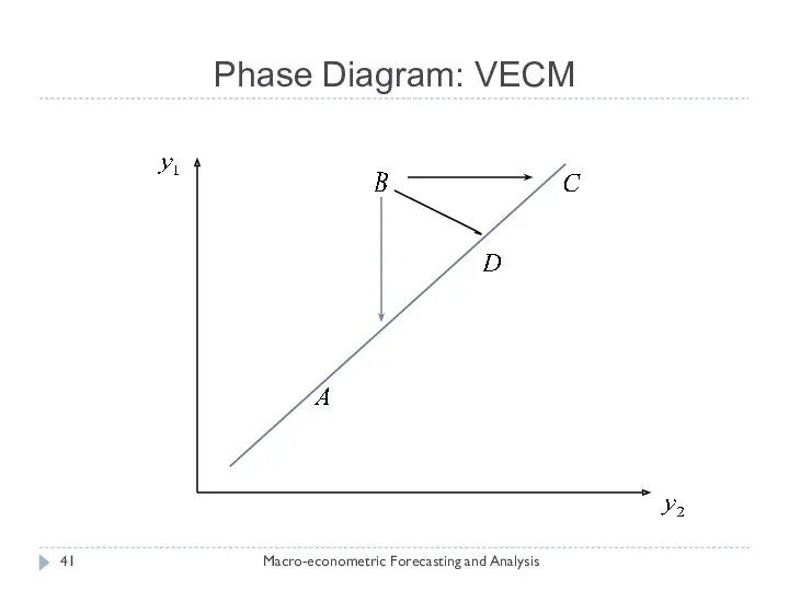
Phase Diagram: VECM
Macro-econometric Forecasting and Analysis
Phase Diagram: VECM
Macro-econometric Forecasting and Analysis
Adjusting Back To Equilibrium
Macro-econometric Forecasting and Analysis
Suppose there is a positive
Adjusting Back To Equilibrium
Macro-econometric Forecasting and Analysis
Suppose there is a positive
Adjustments Are Made by Y1,t
Macro-econometric Forecasting and Analysis
Long-run equilibrium is restored
Adjustments Are Made by Y1,t
Macro-econometric Forecasting and Analysis
Long-run equilibrium is restored
Adjustments Are Made by Y2,t
Macro-econometric Forecasting and Analysis
Long-run equilibrium is restored
Adjustments Are Made by Y2,t
Macro-econometric Forecasting and Analysis
Long-run equilibrium is restored
Adjustments are made by both Y1,t and Y2,t
Macro-econometric Forecasting and Analysis
The
Adjustments are made by both Y1,t and Y2,t
Macro-econometric Forecasting and Analysis
The
VECM = Special VAR
Macro-econometric Forecasting and Analysis
A VECM is actually a
VECM = Special VAR
Macro-econometric Forecasting and Analysis
A VECM is actually a
VECM = Special VAR
Macro-econometric Forecasting and Analysis
VECM = Special VAR
Macro-econometric Forecasting and Analysis
VECM = Special VAR
Macro-econometric Forecasting and Analysis
Obviously, we have a first
VECM = Special VAR
Macro-econometric Forecasting and Analysis
Obviously, we have a first
Multivariate Methods: N > 2
Macro-econometric Forecasting and Analysis
Can easily generalize the
Multivariate Methods: N > 2
Macro-econometric Forecasting and Analysis
Can easily generalize the
VAR with p lags > 1
Macro-econometric Forecasting and Analysis
Allowing for p
VAR with p lags > 1
Macro-econometric Forecasting and Analysis
Allowing for p
Cointegration
Macro-econometric Forecasting and Analysis
If the vector time series yt is assumed
Cointegration
Macro-econometric Forecasting and Analysis
If the vector time series yt is assumed
Granger Representation Theorem
Macro-econometric Forecasting and Analysis
Suppose yt, which can be I(1)
Granger Representation Theorem
Macro-econometric Forecasting and Analysis
Suppose yt, which can be I(1)
Examples: Rank of Long-Run Models
Macro-econometric Forecasting and Analysis
The form of for
Examples: Rank of Long-Run Models
Macro-econometric Forecasting and Analysis
The form of for
Key Implications of the GE Representation Theorem
Macro-econometric Forecasting and Analysis
The Granger-Engle
Key Implications of the GE Representation Theorem
Macro-econometric Forecasting and Analysis
The Granger-Engle
Key Implications of the GE Representation Theorem
Macro-econometric Forecasting and Analysis
If ,
Key Implications of the GE Representation Theorem
Macro-econometric Forecasting and Analysis
If ,
Dealing With Deterministic Components
Macro-econometric Forecasting and Analysis
We can easily extend the
Dealing With Deterministic Components
Macro-econometric Forecasting and Analysis
We can easily extend the
Deterministic Components
Macro-econometric Forecasting and Analysis
Suppose we can decompose these parameters into
Deterministic Components
Macro-econometric Forecasting and Analysis
Suppose we can decompose these parameters into
Deterministic Components
Macro-econometric Forecasting and Analysis
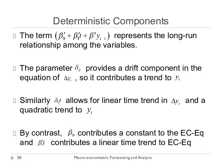
The term represents the long-run relationship among
Deterministic Components
Macro-econometric Forecasting and Analysis
The term represents the long-run relationship among
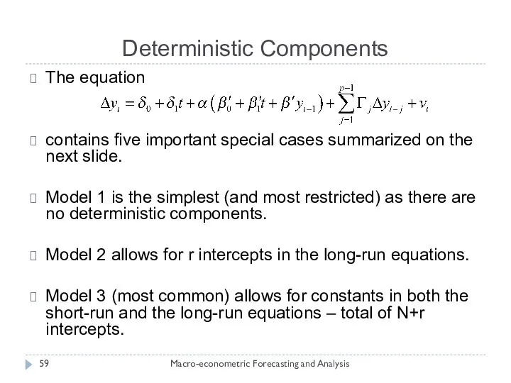
Deterministic Components
Macro-econometric Forecasting and Analysis
The equation
contains five important special cases summarized
Deterministic Components
Macro-econometric Forecasting and Analysis
The equation
contains five important special cases summarized
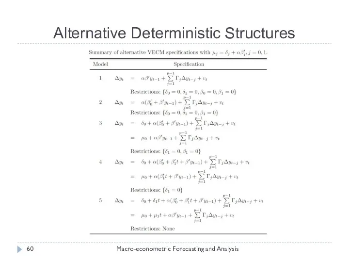
Alternative Deterministic Structures
Macro-econometric Forecasting and Analysis
Alternative Deterministic Structures
Macro-econometric Forecasting and Analysis
Estimating VECM Models
Macro-econometric Forecasting and Analysis
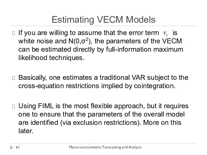
If you are willing to assume
Estimating VECM Models
Macro-econometric Forecasting and Analysis
If you are willing to assume
Three Cases:
Macro-econometric Forecasting and Analysis
VECM is equivalent to the
Three Cases:
Macro-econometric Forecasting and Analysis
VECM is equivalent to the
Reduced Rank (Cointegration) Case: FIML
Macro-econometric Forecasting and Analysis
If cannot be inverted
Reduced Rank (Cointegration) Case: FIML
Macro-econometric Forecasting and Analysis
If cannot be inverted
Reduced Rank Case: Johansen Estimator
Macro-econometric Forecasting and Analysis
We can also use
Reduced Rank Case: Johansen Estimator
Macro-econometric Forecasting and Analysis
We can also use
Zero-Rank Case for
Macro-econometric Forecasting and Analysis
When , the VECM reduces
Zero-Rank Case for
Macro-econometric Forecasting and Analysis
When , the VECM reduces
Identification
Macro-econometric Forecasting and Analysis
The Johansen procedure requires one to normalize the
Identification
Macro-econometric Forecasting and Analysis
The Johansen procedure requires one to normalize the
Identification: Triangular Restrictions
Macro-econometric Forecasting and Analysis
Suppose there are r long-run relationships.
Identification: Triangular Restrictions
Macro-econometric Forecasting and Analysis
Suppose there are r long-run relationships.
Triangular Restrictions
Macro-econometric Forecasting and Analysis
If there are N = 3 variables
Triangular Restrictions
Macro-econometric Forecasting and Analysis
If there are N = 3 variables
Structural Restrictions
Macro-econometric Forecasting and Analysis
Traditional identification methods can also be used
Structural Restrictions
Macro-econometric Forecasting and Analysis
Traditional identification methods can also be used
Open Economy Model
Macro-econometric Forecasting and Analysis
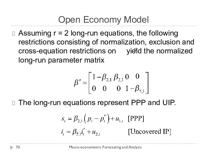
Assuming r = 2 long-run equations,
Open Economy Model
Macro-econometric Forecasting and Analysis
Assuming r = 2 long-run equations,
Cointegration Rank
Macro-econometric Forecasting and Analysis
So far we have taken the rank
Cointegration Rank
Macro-econometric Forecasting and Analysis
So far we have taken the rank
Cointegration Rank: Likelihood Ratio Test
Macro-econometric Forecasting and Analysis
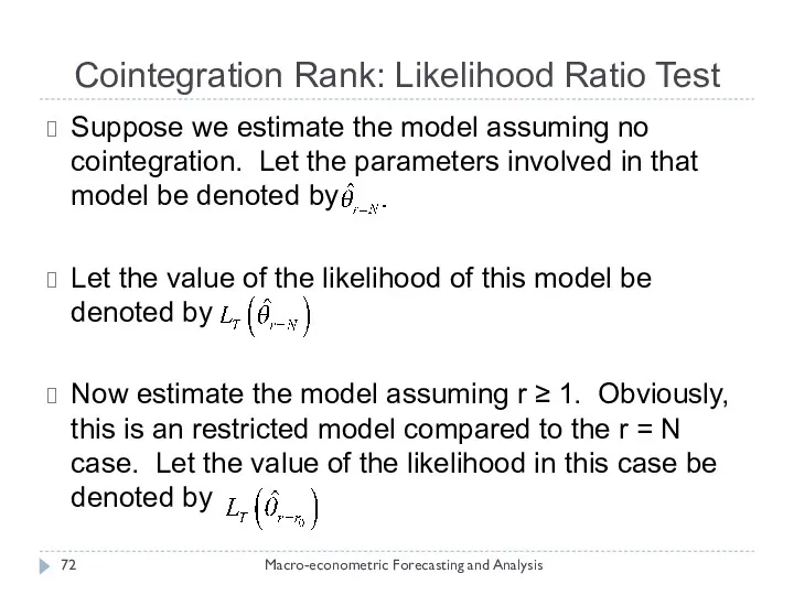
Suppose we estimate the
Cointegration Rank: Likelihood Ratio Test
Macro-econometric Forecasting and Analysis
Suppose we estimate the
Cointegration Rank: Likelihood Ratio Test
Macro-econometric Forecasting and Analysis
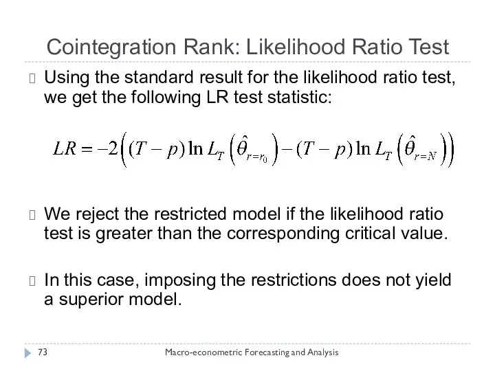
Using the standard result
Cointegration Rank: Likelihood Ratio Test
Macro-econometric Forecasting and Analysis
Using the standard result
Cointegration Rank: Johansen Approach
Macro-econometric Forecasting and Analysis
A numerically equivalent approach was
Cointegration Rank: Johansen Approach
Macro-econometric Forecasting and Analysis
A numerically equivalent approach was
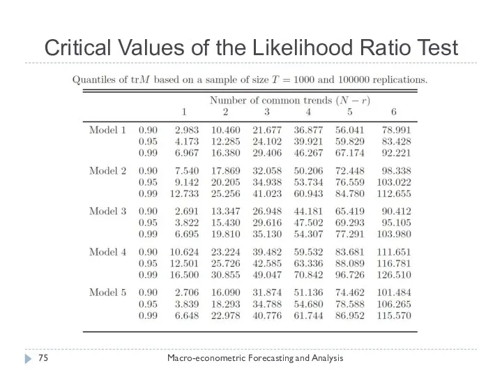
Critical Values of the Likelihood Ratio Test
Macro-econometric Forecasting and Analysis
Critical Values of the Likelihood Ratio Test
Macro-econometric Forecasting and Analysis
Tests on the Cointegrating Vector (Long-Run Parameters)
Macro-econometric Forecasting and Analysis
Hypothesis tests
Tests on the Cointegrating Vector (Long-Run Parameters)
Macro-econometric Forecasting and Analysis
Hypothesis tests
Exogeneity
Macro-econometric Forecasting and Analysis
An important feature of a VECM is that
Exogeneity
Macro-econometric Forecasting and Analysis
An important feature of a VECM is that
Weak versus Strong Exogeneity
Macro-econometric Forecasting and Analysis
If the first channel does
Weak versus Strong Exogeneity
Macro-econometric Forecasting and Analysis
If the first channel does
Example: Exogeneity
Macro-econometric Forecasting and Analysis
Consider the bi-variate term structure model with
Example: Exogeneity
Macro-econometric Forecasting and Analysis
Consider the bi-variate term structure model with
Impulse Response Functions
Macro-econometric Forecasting and Analysis
The dynamics of a VECM can
Impulse Response Functions
Macro-econometric Forecasting and Analysis
The dynamics of a VECM can
Impulse Response Functions: VECM
Macro-econometric Forecasting and Analysis
This VECM can be expressed
Impulse Response Functions: VECM
Macro-econometric Forecasting and Analysis
This VECM can be expressed
Appendices
Appendices
Appendix A: Process moments, key results: AR(1) model with θ <
Appendix A: Process moments, key results: AR(1) model with θ <
Appendix A: Process moments, Simulation of an AR(1) model
Macro-econometric Forecasting and
Appendix A: Process moments, Simulation of an AR(1) model
Macro-econometric Forecasting and
Appendix A: Process moments, key results: AR(1) model with θ =
Appendix A: Process moments, key results: AR(1) model with θ =
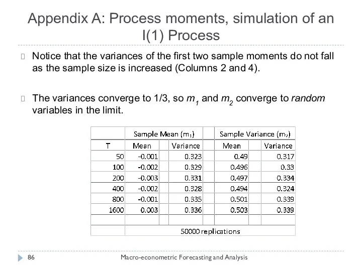
Appendix A: Process moments, simulation of an I(1) Process
Macro-econometric Forecasting and
Appendix A: Process moments, simulation of an I(1) Process
Macro-econometric Forecasting and
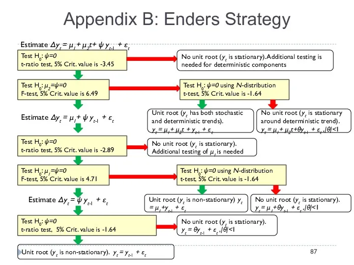
Appendix B: Enders Strategy
Test H0: ψ=0
t-ratio test, 5% Crit. value is
Appendix B: Enders Strategy
Test H0: ψ=0
t-ratio test, 5% Crit. value is
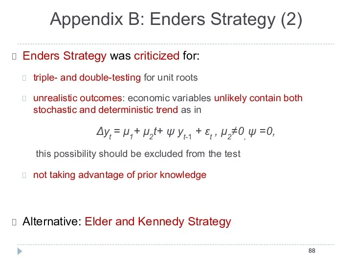
Enders Strategy was criticized for:
triple- and double-testing for unit roots
unrealistic outcomes:
Enders Strategy was criticized for:
triple- and double-testing for unit roots
unrealistic outcomes:
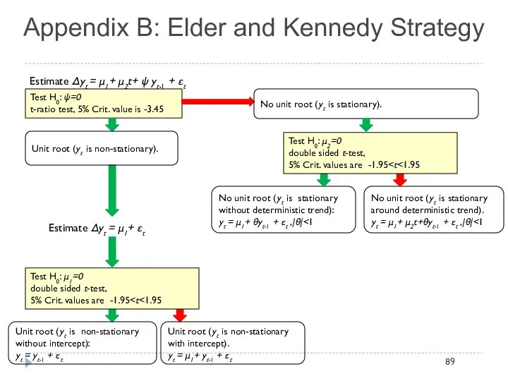
Appendix B: Elder and Kennedy Strategy
Test H0: ψ=0
t-ratio test, 5% Crit.
Appendix B: Elder and Kennedy Strategy
Test H0: ψ=0
t-ratio test, 5% Crit.
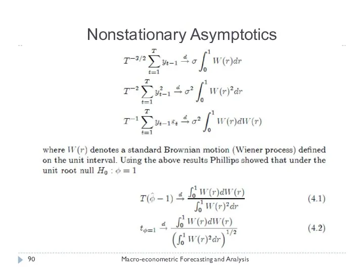
Nonstationary Asymptotics
Macro-econometric Forecasting and Analysis
Nonstationary Asymptotics
Macro-econometric Forecasting and Analysis
 Задачи на вероятность
 Составление задач на сложение и вычитание по одному рисунку
 Логические задачи-шутки на уроках математики в первом классе
 Основные определения реляционной модели данных
 Числа от 11 до 20. Нумерация
 Линейные уравнения с одной переменной
 Реши ребус – отгадай слово
 КВН урок математики в 3 классе
 Таблица значений тригонометрических функций
 Аксиомы параллельных прямых
 Виды треугольников
 Транспортная задача. (Лекции 10,11)
 Моделирование индивидуальной траектории развития одаренных детей по математике в 5-9 классах
 Решение уравнений, сводящихся к квадратным
 Среднее арифметическое, размах и мода. Алгебра. 8 класс
 Анализ систем методами теории массового обслуживания
 Вписанные и описанные окружности. Задания для устного счета. Упражнение 14. 8 класс
 Презентация к уроку математики. Л.Г. Петерсон Умножение и деление на 10, 100 (продолжение)
 Игра Кто хочет стать математиком
 Математический аукцион
 Презентация к уроку по теме Теорема Пифагора
 Оценивание спектральной плотности мощности
 Конспект занятия с презентацией по ФЭМП в средней группе по теме Учимся с Лунтиком!
 проектная задача Доктор Айболит
 Обыкновенные дроби. Сокращение дробей
 Измерительные работы на местности. Творческое название: Геометрия на свежем воздухе
 Вероятность и статистика. 9 класс. Урок № 1
 Практикум по решению стереометрических задач