- Random variables – discrete random variables. Week 6 (2)

Содержание
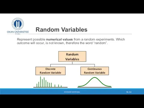
- 2. Random Variables Represent possible numerical values from a random experiments. Which outcome will occur, is not
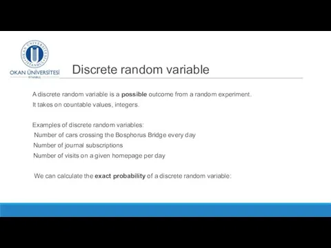
- 3. Discrete random variable A discrete random variable is a possible outcome from a random experiment. It
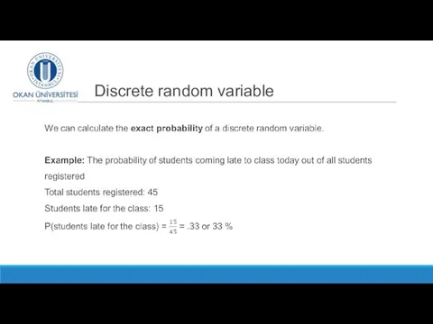
- 4. Discrete random variable
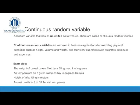
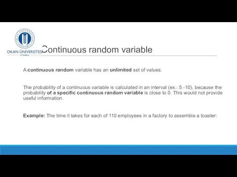
- 5. Continuous random variable A random variable that has an unlimited set of values. Therefore called continuous
- 6. Continuous random variable A continuous random variable has an unlimited set of values. The probability of
- 7. Time, in seconds, it takes 110 employees to assemble a toaster 271 236 294 252 254
- 8. Continuous random variable
- 9. Employee assembly time in seconds Completion time (in seconds) Frequency Relative frequency % 220 – 229
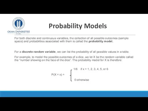
- 10. Probability Models For both discrete and continuous variables, the collection of all possible outcomes (sample space)
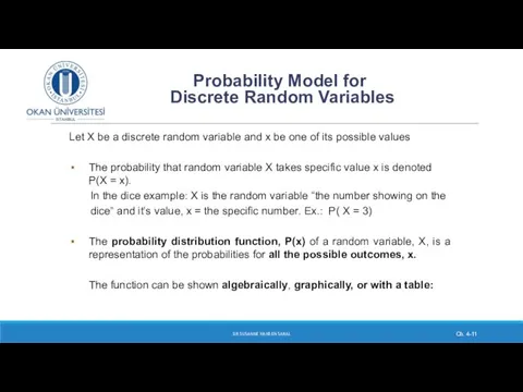
- 11. Ch. 4- DR SUSANNE HANSEN SARAL Probability Model for Discrete Random Variables Let X be a
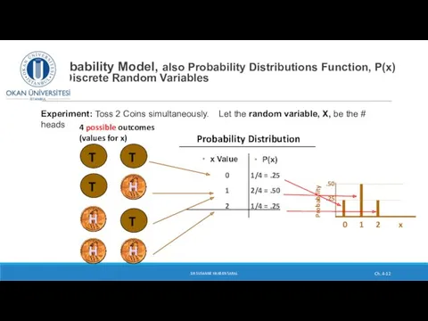
- 12. Ch. 4- DR SUSANNE HANSEN SARAL Probability Model, also Probability Distributions Function, P(x) for Discrete Random
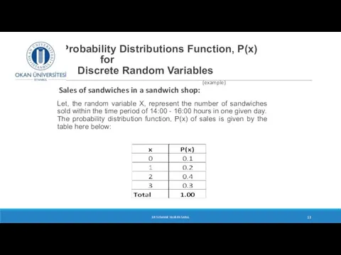
- 13. Probability Distributions Function, P(x) for Discrete Random Variables (example) Sales of sandwiches in a sandwich shop:
- 14. Graphical illustration of the probability distribution of sandwich sales between 14:00 -16:00 hours DR SUSANNE HANSEN
- 15. Requirements for a probability distribution of a discrete random variable DR SUSANNE HANSEN SARAL Ch. 4-
- 16. Cumulative Probability Function DR SUSANNE HANSEN SARAL Ch. 4- (continued) X Value P(x) F(x) 0 0.25
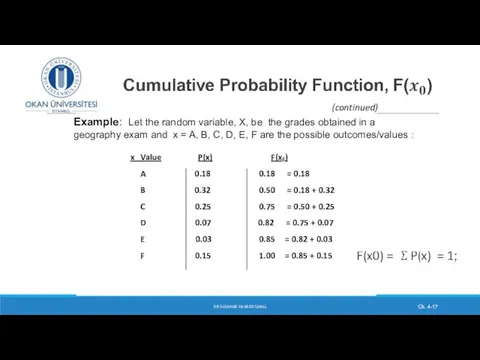
- 17. DR SUSANNE HANSEN SARAL Ch. 4- (continued) x Value P(x) F(x0) A 0.18 0.18 = 0.18
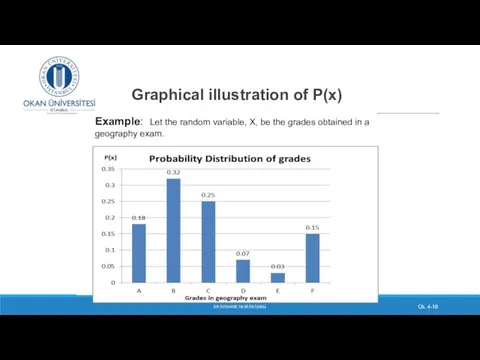
- 18. Graphical illustration of P(x) DR SUSANNE HANSEN SARAL Ch. 4- Example: Let the random variable, X,
- 19. Graphical illustration of F(x0) Cumulative probability distribution, Ogive DR SUSANNE HANSEN SARAL Ch. 4- Example: Let
- 20. Cumulative Probability Function, F(x0) Practical application DR SUSANNE HANSEN SARAL The cumulative probability distribution can be
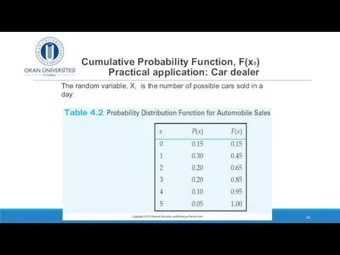
- 21. Cumulative Probability Function, F(x0) Practical application: Car dealer DR SUSANNE HANSEN SARAL The random variable, X,
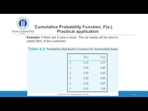
- 22. Cumulative Probability Function, F(x0) Practical application DR SUSANNE HANSEN SARAL Example: If there are 3 cars
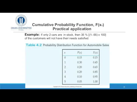
- 23. Cumulative Probability Function, F(x0) Practical application DR SUSANNE HANSEN SARAL Example: If only 2 cars are
- 24. 3/9/2017 DR SUSANNE HANSEN SARAL
- 25. Cumulative probability - solution DR SUSANNE HANSEN SARAL
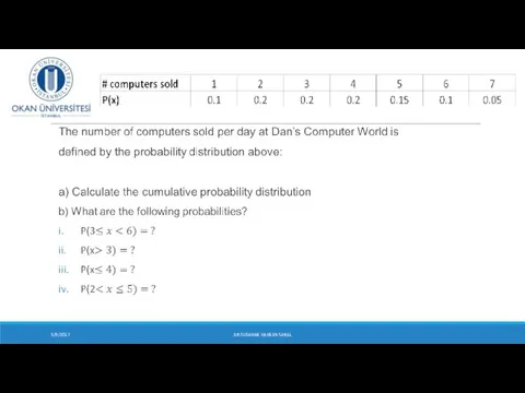
- 26. Exercise In a geography exam the grade students obtained is the random variable X. It has
- 27. Cumulative probabilities - exercise Based on this, calculate the following: The cumulative probability distribution of X,
- 28. Properties of Discrete Random Variables The measurements of central tendency and variation for discrete random variables:
- 29. Expectations
- 30. Expected Value of a discrete random variable X: Example: Toss 2 coins, random variable, X =
- 31. Properties of Discrete Random Variables Expected Value (or mean) of a discrete random variable X: We
- 32. Expected value So, the expected value, E[X], of a discrete random variable is found by multiplying
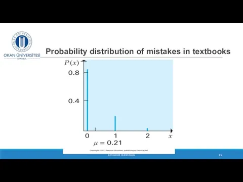
- 33. Concept of expected value of a random variable A review of university textbooks reveals that 81
- 34. Expected value – calculation (example) Find the expected mean number of mistakes on pages: = (0)(.81)+(1)(.17)+(2)(.02)
- 35. Probability distribution of mistakes in textbooks DR SUSANNE HANSEN SARAL
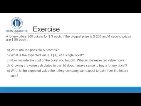
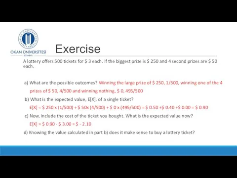
- 36. Exercise A lottery offers 500 tickets for $ 3 each. If the biggest prize is $
- 37. Exercise A lottery offers 500 tickets for $ 3 each. If the biggest prize is $
- 39. Скачать презентацию
Random Variables
Represent possible numerical values from a random experiments. Which outcome
Random Variables
Represent possible numerical values from a random experiments. Which outcome
Discrete random variable
A discrete random variable is a possible outcome
Discrete random variable
A discrete random variable is a possible outcome
Discrete random variable
Discrete random variable
Continuous random variable
A random variable that has an unlimited set of
Continuous random variable
A random variable that has an unlimited set of
Continuous random variable
A continuous random variable has an unlimited set of
Continuous random variable
A continuous random variable has an unlimited set of
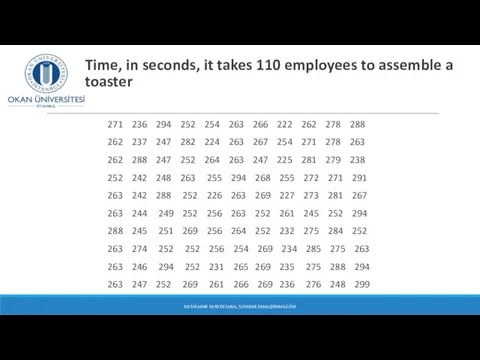
Time, in seconds, it takes 110 employees to assemble a
Time, in seconds, it takes 110 employees to assemble a
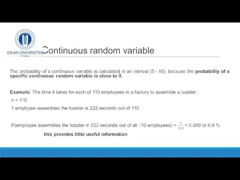
Continuous random variable
Continuous random variable
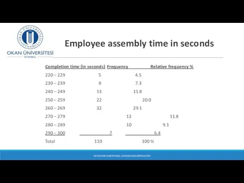
Employee assembly time in seconds
Completion time (in seconds) Frequency Relative frequency
Employee assembly time in seconds
Completion time (in seconds) Frequency Relative frequency
Probability Models
For both discrete and continuous variables, the collection of
Probability Models
For both discrete and continuous variables, the collection of
Ch. 4-
DR SUSANNE HANSEN SARAL
Probability Model for
Discrete Random
Ch. 4-
DR SUSANNE HANSEN SARAL
Probability Model for
Discrete Random
Ch. 4-
DR SUSANNE HANSEN SARAL
Probability Model, also Probability Distributions Function,
Ch. 4-
DR SUSANNE HANSEN SARAL
Probability Model, also Probability Distributions Function,
Probability Distributions Function, P(x) for Discrete Random Variables
(example)
Sales of
Probability Distributions Function, P(x) for Discrete Random Variables
(example)
Sales of
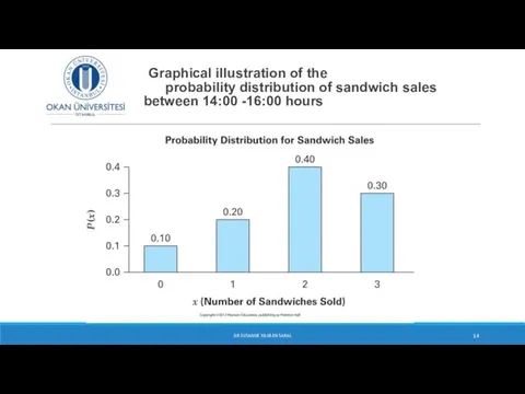
Graphical illustration of the probability distribution of sandwich sales
between
Graphical illustration of the probability distribution of sandwich sales between
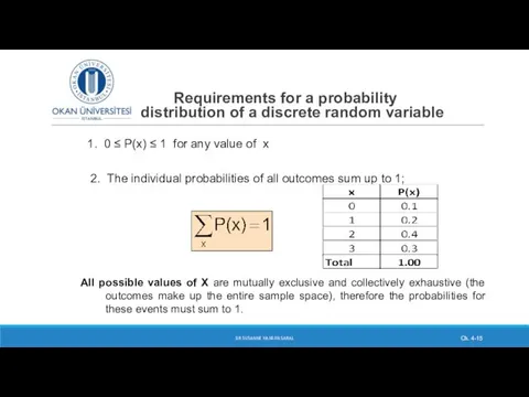
Requirements for a probability distribution of a discrete random variable
DR
Requirements for a probability distribution of a discrete random variable
DR
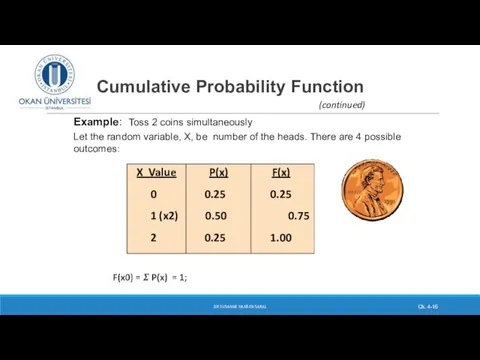
Cumulative Probability Function
DR SUSANNE HANSEN SARAL
Ch. 4-
(continued)
X Value P(x) F(x)
Cumulative Probability Function
DR SUSANNE HANSEN SARAL
Ch. 4-
(continued)
X Value P(x) F(x)
DR SUSANNE HANSEN SARAL
Ch. 4-
(continued)
x Value P(x) F(x0)
A 0.18
DR SUSANNE HANSEN SARAL
Ch. 4-
(continued)
x Value P(x) F(x0)
A 0.18
Graphical illustration of P(x)
DR SUSANNE HANSEN SARAL
Ch. 4-
Example: Let the
Graphical illustration of P(x)
DR SUSANNE HANSEN SARAL
Ch. 4-
Example: Let the
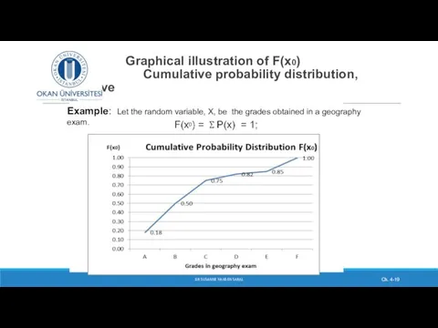
Graphical illustration of F(x0)
Cumulative probability distribution, Ogive
DR SUSANNE HANSEN
Graphical illustration of F(x0)
Cumulative probability distribution, Ogive
DR SUSANNE HANSEN
Cumulative Probability Function, F(x0)
Practical application
DR SUSANNE HANSEN SARAL
The cumulative
Cumulative Probability Function, F(x0)
Practical application
DR SUSANNE HANSEN SARAL
The cumulative
Cumulative Probability Function, F(x0)
Practical application: Car dealer
DR SUSANNE HANSEN
Cumulative Probability Function, F(x0)
Practical application: Car dealer
DR SUSANNE HANSEN
Cumulative Probability Function, F(x0)
Practical application
DR SUSANNE HANSEN SARAL
Example: If
Cumulative Probability Function, F(x0)
Practical application
DR SUSANNE HANSEN SARAL
Example: If
Cumulative Probability Function, F(x0)
Practical application
DR SUSANNE HANSEN SARAL
Example: If
Cumulative Probability Function, F(x0)
Practical application
DR SUSANNE HANSEN SARAL
Example: If
3/9/2017
DR SUSANNE HANSEN SARAL
3/9/2017
DR SUSANNE HANSEN SARAL
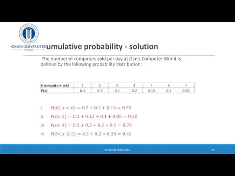
Cumulative probability - solution
DR SUSANNE HANSEN SARAL
Cumulative probability - solution
DR SUSANNE HANSEN SARAL
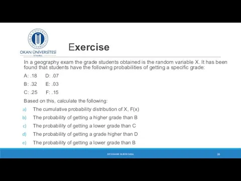
Exercise
In a geography exam the grade students obtained is the random
Exercise
In a geography exam the grade students obtained is the random
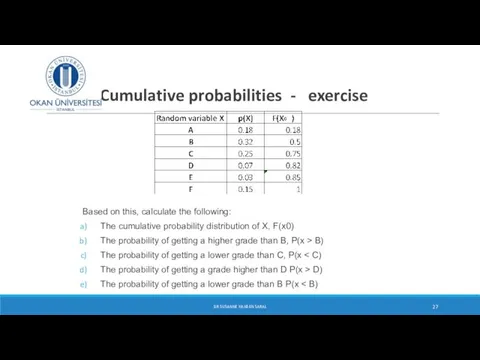
Cumulative probabilities - exercise
Based on this, calculate the following:
The cumulative probability
Cumulative probabilities - exercise
Based on this, calculate the following:
The cumulative probability
Properties of
Discrete Random Variables
The measurements of central tendency and variation
Properties of
Discrete Random Variables
The measurements of central tendency and variation
Expectations
Expectations
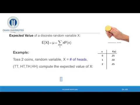
Expected Value of a discrete random variable X:
Example:
Toss 2 coins,
Expected Value of a discrete random variable X:
Example:
Toss 2 coins,
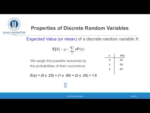
Properties of Discrete Random Variables
Expected Value (or mean)
Properties of Discrete Random Variables
Expected Value (or mean)
![Expected value So, the expected value, E[X], of a discrete](/_ipx/f_webp&q_80&fit_contain&s_1440x1080/imagesDir/jpg/14375/slide-31.jpg)
Expected value
So, the expected value, E[X], of a discrete random
Expected value
So, the expected value, E[X], of a discrete random
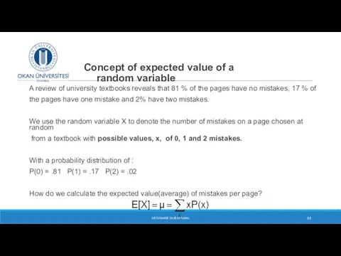
Concept of expected value of a
random variable
A review of university
Concept of expected value of a
random variable
A review of university
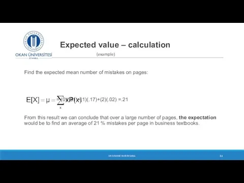
Expected value – calculation
(example)
Find the expected mean number of mistakes
Expected value – calculation
(example)
Find the expected mean number of mistakes
Probability distribution of mistakes in textbooks
DR SUSANNE HANSEN SARAL
Probability distribution of mistakes in textbooks
DR SUSANNE HANSEN SARAL
Exercise
A lottery offers 500 tickets for $ 3 each. If
Exercise
A lottery offers 500 tickets for $ 3 each. If
Exercise
A lottery offers 500 tickets for $ 3 each. If
Exercise
A lottery offers 500 tickets for $ 3 each. If
 Применение производной и интегралов в различных областях биологии и химии
 Теорема Пифагора
 Самостоятельная работа
 Түзусызықты теңайнымалы қозғалыс, үдеу
 Из истории геометрических терминов
 Презентация Сочетательное свойство сложения
 Решение задач на смеси и сплавы
 Интеллектуальные информационные системы. Лекция 6. Нечеткая логика. Математические основы
 Решение задач по теме Параллельность плоскостей. Тетраэдр и параллелепипед
 Повторення вивченого. Додаткові вправи. Урок №136
 Игра – самый умный математик. 6 класс
 Расстояние между двумя точками. Масштаб
 Таблица истинности для импликации
 Нестандартные способы решения тригонометрических уравнений
 Площади параллелограмма, треугольника и трапеции. Урок 21-22
 Графоаналитические методы оценки параметров распределения (лекция 5)
 Додавання і віднімання раціональних чисел
 П’єр де Ферма (1601-1665)
 Презентация к уроку Задача 1 класс
 Рішення рівнянь
 Делители и кратные (часть 3)
 Тест по теме: четырехугольники
 Решение систем линейных уравнений методом Крамера, методом Гаусса и матричным методом (вопросы)
 Дроби. Нахождение части числа. Нахождение целого по его части.
 Умножение и деление положительных и отрицательных чисел
 Меньше или больше. Демонстрационный материал. 5 класс
 ПРЕЗЕНТАЦИЯ Умножение многозначного числа на однозначное (закрепление)
 Презентация ТАНГРАМ Животные