- T PM N 2019/2020 : Solving the Schr¨odingerequation

Содержание
- 2. TPMN 2019/2020 : Solving the Schr¨odinger equation e M. Alouani, mebarek.alouani@ipcms.unistra.fr, IPCMS e H. Bulou, herve.bulou@ipcms.unistra.fr,
- 3. TPMN 2019/2020 : Solving the Schr¨odinger equation e M. Alouani, mebarek.alouani@ipcms.unistra.fr, IPCMS e H. Bulou, herve.bulou@ipcms.unistra.fr,
- 4. TPMN 2019/2020 : Solving the Schr¨odinger equation e M. Alouani, mebarek.alouani@ipcms.unistra.fr, IPCMS e H. Bulou, herve.bulou@ipcms.unistra.fr,
- 5. TPMN 2019/2020 : Solving the Schr¨odinger equation e M. Alouani, mebarek.alouani@ipcms.unistra.fr, IPCMS e H. Bulou, herve.bulou@ipcms.unistra.fr,
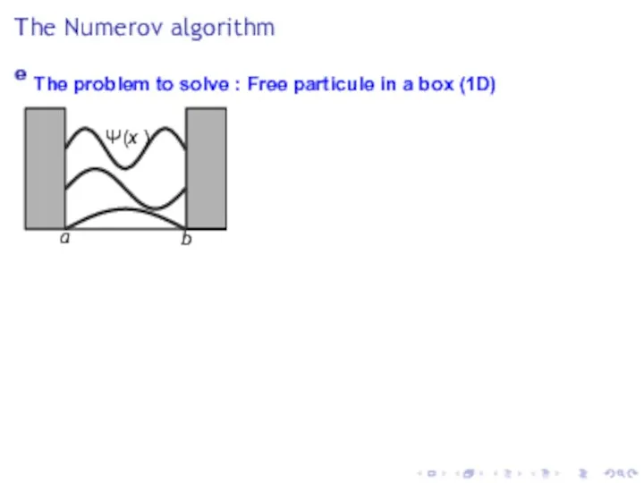
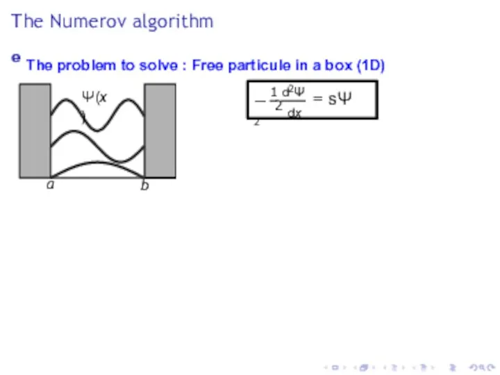
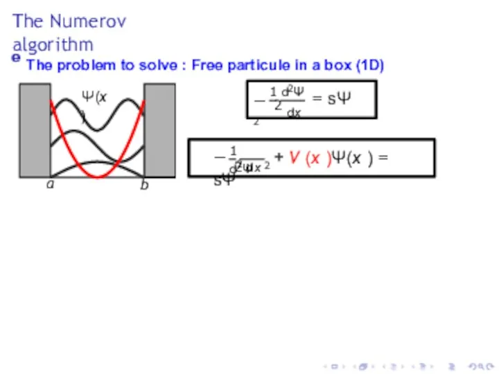
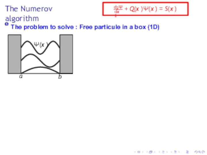
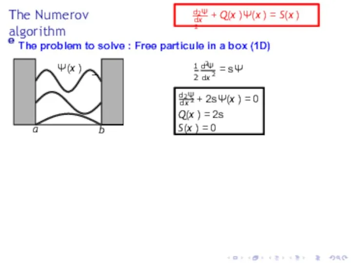
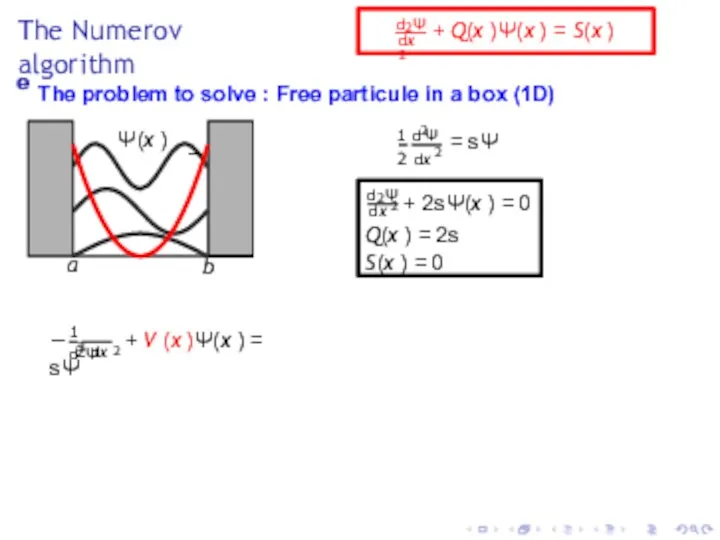
- 6. The Numerov algorithm e The problem to solve : Free particule in a box (1D) Ψ(x
- 7. The Numerov algorithm e The problem to solve : Free particule in a box (1D) Ψ(x
- 8. The Numerov algorithm e The problem to solve : Free particule in a box (1D) Ψ(x
- 9. The Numerov algorithm e The problem to solve : Free particule in a box (1D) Ψ(x
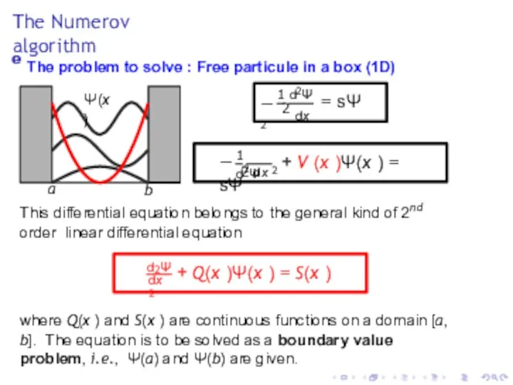
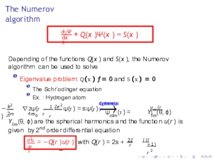
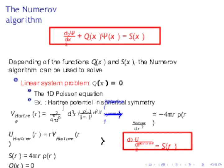
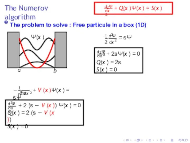
- 10. The Numerov algorithm dx 2 d2Ψ + Q(x )Ψ(x ) = S(x ) 2 − ∇
- 11. The Numerov algorithm dx 2 d2Ψ + Q(x )Ψ(x ) = S(x ) Depending of the
- 12. The Numerov algorithm e The problem to solve : Free particule in a box (1D) Ψ(x
- 13. The Numerov algorithm e The problem to solve : Free particule in a box (1D) a
- 14. The Numerov algorithm e The problem to solve : Free particule in a box (1D) a
- 15. The Numerov algorithm e The problem to solve : Free particule in a box (1D) a
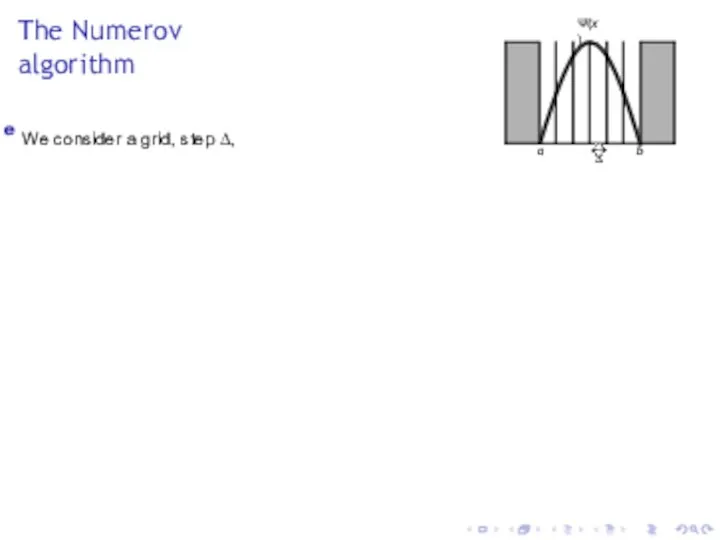
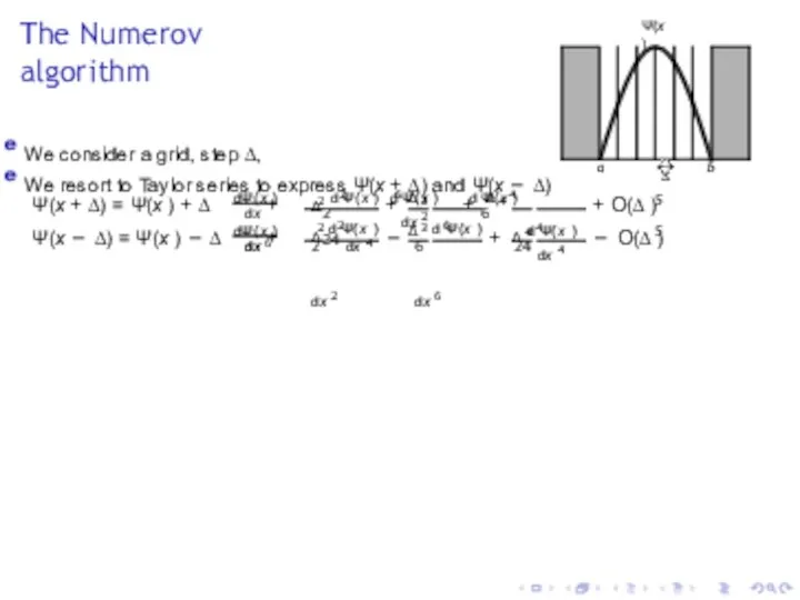
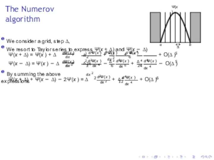
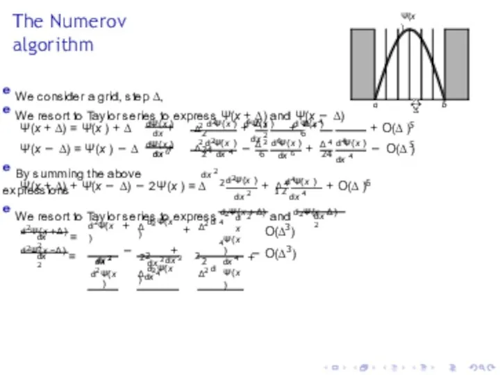
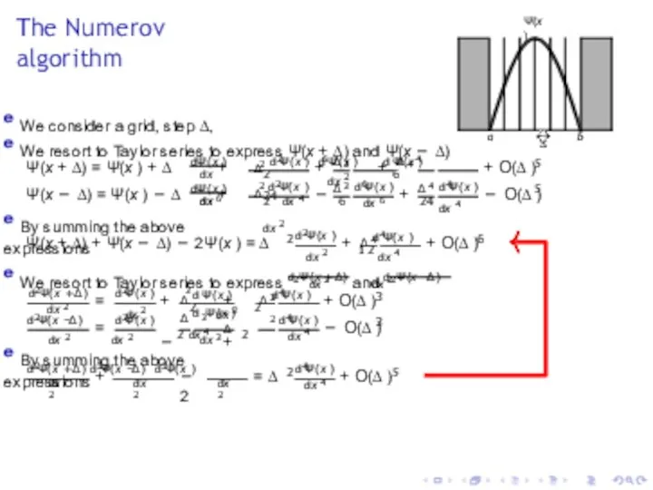
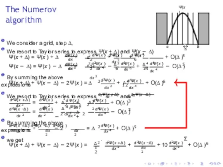
- 16. The Numerov algorithm Ψ(x ) a b ∆ e We consider a grid, step ∆,
- 17. The Numerov algorithm Ψ(x ) a b ∆ e We consider a grid, step ∆, e
- 18. The Numerov algorithm Ψ(x ) a b ∆ e We consider a grid, step ∆, e
- 19. The Numerov algorithm Ψ(x ) a b ∆ e We consider a grid, step ∆, e
- 20. The Numerov algorithm Ψ(x ) a b ∆ e We consider a grid, step ∆, e
- 21. The Numerov algorithm Ψ(x ) a b ∆ e We consider a grid, step ∆, e
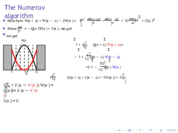
- 22. The Numerov algorithm Ψ(x ) a b ∆ Now from Ψ(x + ∆) + Ψ(x −
- 23. The Numerov algorithm Ψ(x ) a b ∆ Σ ∆2 12 Σ 1 + Q(x +
- 24. The Numerov algorithm Ψ(x ) a b ∆ Σ ∆2 12 Σ 1 + Q(x +
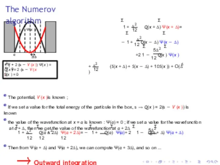
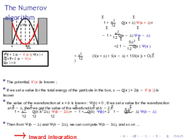
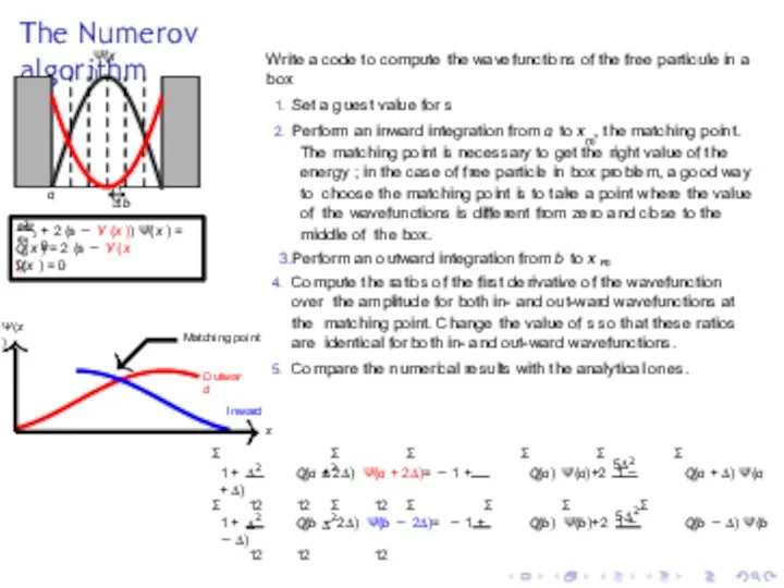
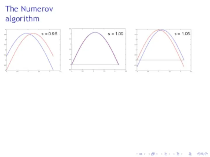
- 25. The Numerov algorithm Ψ(x ) a b ∆ 2 d Ψ dx 2 + 2 (s
- 26. The Numerov algorithm s = 0.95 s = 1.00 s = 1.05
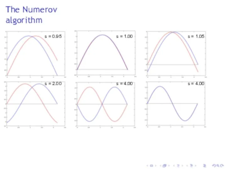
- 27. The Numerov algorithm s = 0.95 s = 1.00 s = 1.05 s = 2.00 s
- 29. Скачать презентацию
TPMN 2019/2020 : Solving the Schr¨odinger equation
e M. Alouani, mebarek.alouani@ipcms.unistra.fr, IPCMS
e
TPMN 2019/2020 : Solving the Schr¨odinger equation
e M. Alouani, mebarek.alouani@ipcms.unistra.fr, IPCMS
e
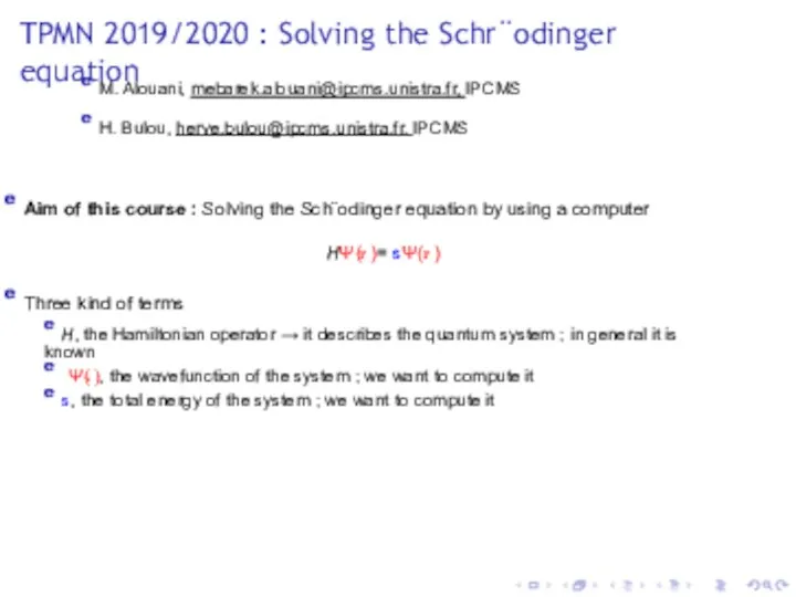
TPMN 2019/2020 : Solving the Schr¨odinger equation
e M. Alouani, mebarek.alouani@ipcms.unistra.fr, IPCMS
e
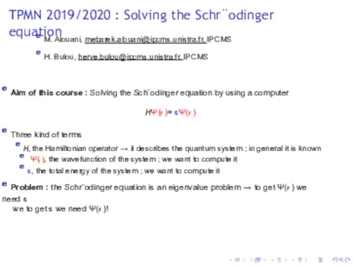
TPMN 2019/2020 : Solving the Schr¨odinger equation
e M. Alouani, mebarek.alouani@ipcms.unistra.fr, IPCMS
e
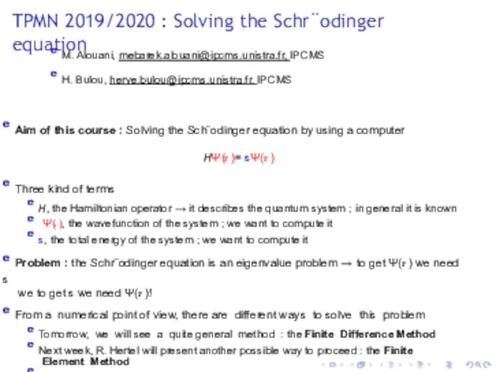
TPMN 2019/2020 : Solving the Schr¨odinger equation
e M. Alouani, mebarek.alouani@ipcms.unistra.fr, IPCMS
e
TPMN 2019/2020 : Solving the Schr¨odinger equation
e M. Alouani, mebarek.alouani@ipcms.unistra.fr, IPCMS
e
TPMN 2019/2020 : Solving the Schr¨odinger equation
e M. Alouani, mebarek.alouani@ipcms.unistra.fr, IPCMS
e
TPMN 2019/2020 : Solving the Schr¨odinger equation
e M. Alouani, mebarek.alouani@ipcms.unistra.fr, IPCMS
e
The Numerov algorithm
e The problem to solve : Free particule in
The Numerov algorithm
e The problem to solve : Free particule in
The Numerov algorithm
e The problem to solve : Free particule in
The Numerov algorithm
e The problem to solve : Free particule in
The Numerov algorithm
e The problem to solve : Free particule in
The Numerov algorithm
e The problem to solve : Free particule in
The Numerov algorithm
e The problem to solve : Free particule in
The Numerov algorithm
e The problem to solve : Free particule in
The Numerov algorithm
dx 2
d2Ψ + Q(x )Ψ(x ) = S(x )
2
− ∇
The Numerov algorithm
dx 2
d2Ψ + Q(x )Ψ(x ) = S(x )
2
− ∇
The Numerov algorithm
dx 2
d2Ψ + Q(x )Ψ(x ) = S(x )
Depending
The Numerov algorithm
dx 2
d2Ψ + Q(x )Ψ(x ) = S(x )
Depending
The Numerov algorithm
e The problem to solve : Free particule in
The Numerov algorithm
e The problem to solve : Free particule in
The Numerov algorithm
e The problem to solve : Free particule in
The Numerov algorithm
e The problem to solve : Free particule in
The Numerov algorithm
e The problem to solve : Free particule in
The Numerov algorithm
e The problem to solve : Free particule in
The Numerov algorithm
e The problem to solve : Free particule in
The Numerov algorithm
e The problem to solve : Free particule in
The Numerov algorithm
Ψ(x )
a
b
∆
e We consider a grid, step ∆,
The Numerov algorithm
Ψ(x )
a
b
∆
e We consider a grid, step ∆,
The Numerov algorithm
Ψ(x )
a
b
∆
e We consider a grid, step ∆,
e We
The Numerov algorithm
Ψ(x )
a
b
∆
e We consider a grid, step ∆,
e We
The Numerov algorithm
Ψ(x )
a
b
∆
e We consider a grid, step ∆,
e We
The Numerov algorithm
Ψ(x )
a
b
∆
e We consider a grid, step ∆,
e We
The Numerov algorithm
Ψ(x )
a
b
∆
e We consider a grid, step ∆,
e We
The Numerov algorithm
Ψ(x )
a
b
∆
e We consider a grid, step ∆,
e We
The Numerov algorithm
Ψ(x )
a
b
∆
e We consider a grid, step ∆,
e We
The Numerov algorithm
Ψ(x )
a
b
∆
e We consider a grid, step ∆,
e We
The Numerov algorithm
Ψ(x )
a
b
∆
e We consider a grid, step ∆,
e We
The Numerov algorithm
Ψ(x )
a
b
∆
e We consider a grid, step ∆,
e We
The Numerov algorithm
Ψ(x )
a
b
∆
Now from Ψ(x + ∆) + Ψ(x −
The Numerov algorithm
Ψ(x )
a
b
∆
Now from Ψ(x + ∆) + Ψ(x −
The Numerov algorithm
Ψ(x )
a b
∆
Σ
∆2
12
Σ
1 + Q(x + ∆) Ψ(x + ∆)=
Σ
∆2
Σ
− 1
The Numerov algorithm
Ψ(x )
a b
∆
Σ
∆2
12
Σ
1 + Q(x + ∆) Ψ(x + ∆)=
Σ
∆2
Σ
− 1
The Numerov algorithm
Ψ(x )
a b
∆
Σ
∆2
12
Σ
1 + Q(x + ∆) Ψ(x + ∆)=
Σ
∆2
Σ
− 1
The Numerov algorithm
Ψ(x )
a b
∆
Σ
∆2
12
Σ
1 + Q(x + ∆) Ψ(x + ∆)=
Σ
∆2
Σ
− 1
The Numerov algorithm
Ψ(x )
a b
∆
2
d Ψ
dx 2
+ 2 (s − V (x
The Numerov algorithm
Ψ(x )
a b
∆
2
d Ψ
dx 2
+ 2 (s − V (x
The Numerov algorithm
s = 0.95
s = 1.00
s = 1.05
The Numerov algorithm
s = 0.95
s = 1.00
s = 1.05
The Numerov algorithm
s = 0.95
s = 1.00
s = 1.05
s = 2.00
s
The Numerov algorithm
s = 0.95
s = 1.00
s = 1.05
s = 2.00
s
 Решение системы способом подстановки. 7 класс
 Адаптивные фильтры. Практическое применение (1)
 Повторение материала по теме Обыкновенные дроби. 6 класс
 Площадь трапеции
 Презентация Развитие математических способностей у детей дошкольного возраста
 Математика. 1 класс. Урок 13. Число два. Цифра 2. Презентация
 Внеклассное мероприятие по информатике и математике. Викторина
 Математика. 1 класс. Урок 99. Сложение и вычитание в пределах 20 - Презентация
 Функции, пределы, непрерывности
 Методы искусственного базиса при решении ЗЛП. Лекция 3
 Многоугольники. Четырёхугольники
 Basics of functions and their graphs
 В стране сенсорики
 Геометрические головоломки
 Платоновы тела
 Презентация к уроку по теме Закрепление изученного. Единицы измерения времени
 Кратные интегралы. (Лекция 3)
 Математическая мозаика
 Деление на десятичную дробь. Правило деления
 Линейные уравнения (Алгебра – 7 класс). Электронный учебник
 Дифференциальное исчисление функции одной переменной
 Синус, косинус и тангенс острого угла прямоугольного треугольника
 Музыкальные инструменты для детей
 презентация к уроку математики по теме Периметр 2 класс по программе Школа 2100
 Команда Умники и умницы
 Образование чисел из одного десятка и нескольких единиц
 Применение игровых технологий для развития и коррекции познавательных процессов на уроках математики в начальных классах
 Умножение и деление