- Review for midterm exam II

Содержание
- 2. The Line Balancing Problem The problem is to arrange the individual tasks at the workstations so
- 3. Line Balancing The actual cycle time which is the maximum workload assigned to a workstation should
- 4. If the demand is 12 cases per 8-hour day, compute a) the required cycle time b)
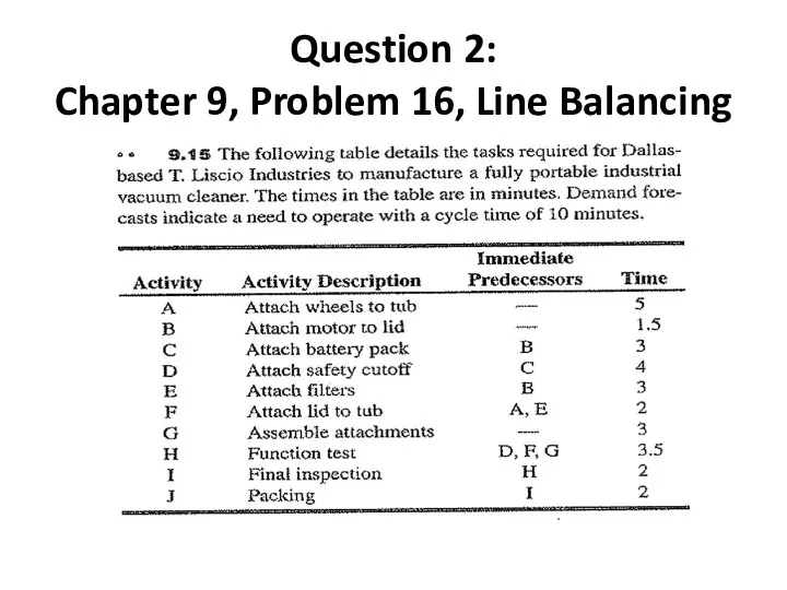
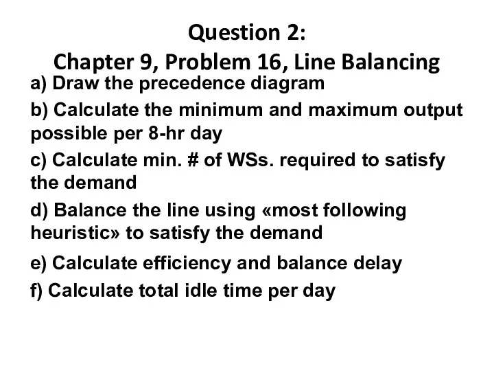
- 5. Question 2: Chapter 9, Problem 16, Line Balancing
- 6. Question 2: Chapter 9, Problem 16, Line Balancing a) Draw the precedence diagram b) Calculate the
- 7. Inventory Management EOQ Model
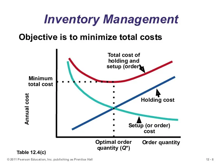
- 8. © 2011 Pearson Education, Inc. publishing as Prentice Hall Inventory Management Objective is to minimize total
- 9. Inventory Management EOQ Model
- 10. EOQ Model Equations D = Demand per year S = Setup (order) cost per order H
- 11. Question 3, EOQ The ABC store needs 1000 coffee makers per year. Ordering cost is $100
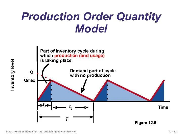
- 12. © 2011 Pearson Education, Inc. publishing as Prentice Hall Production Order Quantity Model Figure 12.6
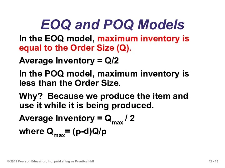
- 13. EOQ and POQ Models In the EOQ model, maximum inventory is equal to the Order Size
- 14. POQ Model D – annual demand S – Setup cost H – Holding cost d –
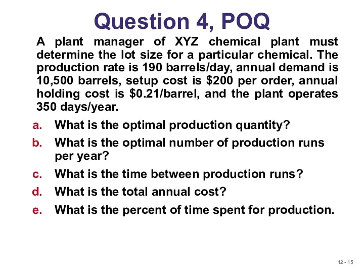
- 15. Question 4, POQ A plant manager of XYZ chemical plant must determine the lot size for
- 16. Question 5:Chapter 12, Problem 20, POQ
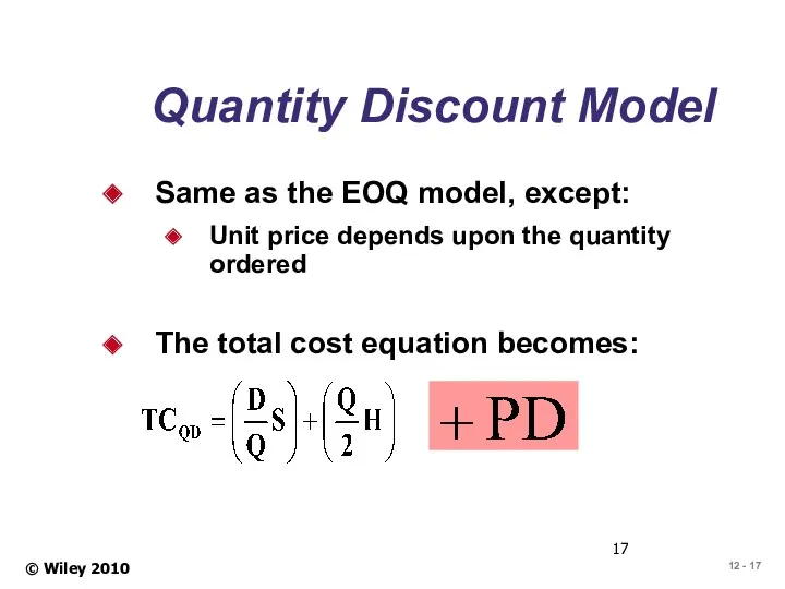
- 17. © Wiley 2010 Quantity Discount Model Same as the EOQ model, except: Unit price depends upon
- 18. Question 6: Quantity Discount Model ABC Sport store is considering going to a different hat supplier.
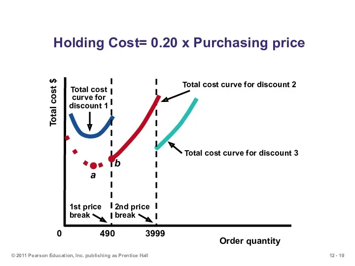
- 19. © 2011 Pearson Education, Inc. publishing as Prentice Hall Holding Cost= 0.20 x Purchasing price
- 20. Question 7: Quantity Discount Model A company has a chance to reduce their inventory ordering costs
- 21. Total Cost with Constant Holding Costs In this case there is a single minimum point; all
- 22. Question 8: Reorder Point for Variable Demand The manager of a carpet store wants to determine
- 23. Demand per day is variable and lead time (in days) is constant ROP =(Average daily demand)
- 24. © 2011 Pearson Education, Inc. publishing as Prentice Hall
- 25. Question 9: Aggregate Production Planning © 2011 Pearson Education, Inc. publishing as Prentice Hall ABC Company
- 26. Question 9: Aggregate Production Planning Which of the following production plans is better: Plan A–chase demand
- 27. a) Chase Demand © 2011 Pearson Education, Inc. publishing as Prentice Hall
- 29. Скачать презентацию
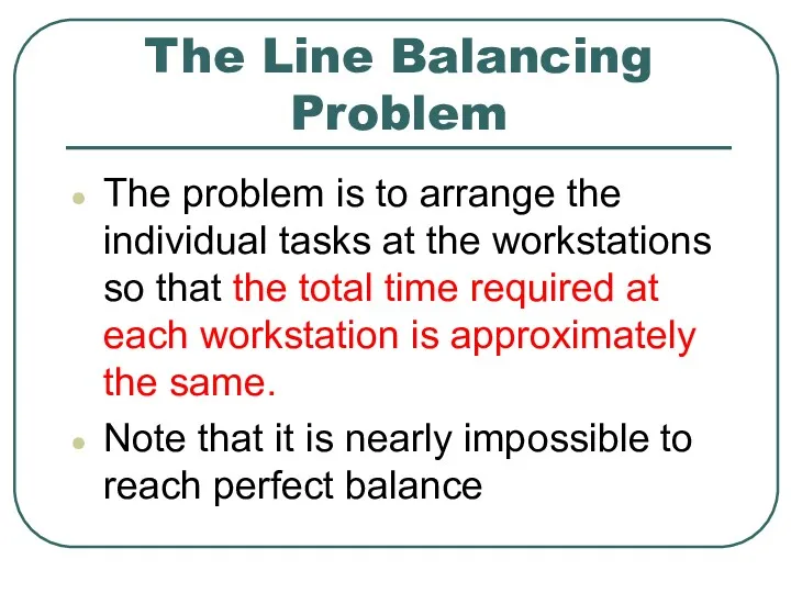
The Line Balancing Problem
The problem is to arrange the individual tasks
The Line Balancing Problem
The problem is to arrange the individual tasks
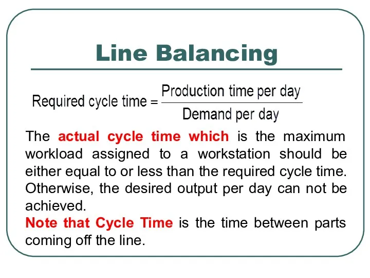
Line Balancing
The actual cycle time which is the maximum workload assigned
Line Balancing
The actual cycle time which is the maximum workload assigned
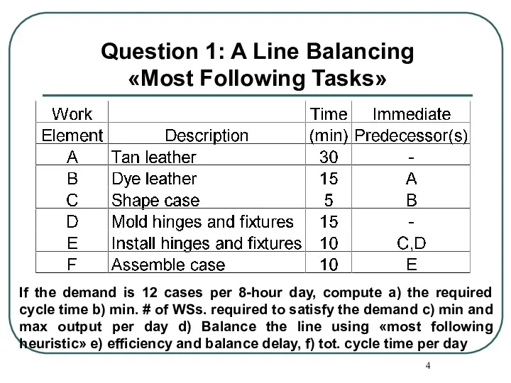
If the demand is 12 cases per 8-hour day, compute a)
If the demand is 12 cases per 8-hour day, compute a)
Question 2:
Chapter 9, Problem 16, Line Balancing
Question 2:
Chapter 9, Problem 16, Line Balancing
Question 2:
Chapter 9, Problem 16, Line Balancing
a) Draw the precedence diagram
b)
Question 2:
Chapter 9, Problem 16, Line Balancing
a) Draw the precedence diagram
b)
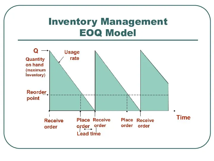
Inventory Management
EOQ Model
Inventory Management
EOQ Model
© 2011 Pearson Education, Inc. publishing as Prentice Hall
Inventory Management
Objective is
© 2011 Pearson Education, Inc. publishing as Prentice Hall
Inventory Management
Objective is

Inventory Management
EOQ Model
Inventory Management
EOQ Model

EOQ Model Equations
D = Demand per year
S = Setup (order) cost
EOQ Model Equations
D = Demand per year
S = Setup (order) cost
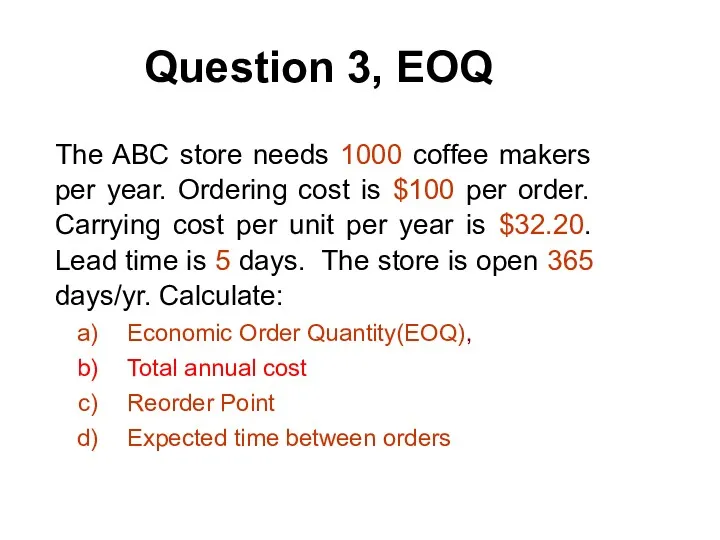
Question 3, EOQ
The ABC store needs 1000 coffee makers per year.
Question 3, EOQ
The ABC store needs 1000 coffee makers per year.
© 2011 Pearson Education, Inc. publishing as Prentice Hall
Production Order Quantity
© 2011 Pearson Education, Inc. publishing as Prentice Hall
Production Order Quantity
EOQ and POQ Models
In the EOQ model, maximum inventory is equal
EOQ and POQ Models
In the EOQ model, maximum inventory is equal
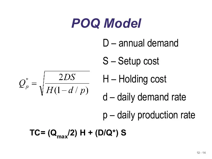
POQ Model
D – annual demand
S – Setup cost
H – Holding cost
d
POQ Model
D – annual demand
S – Setup cost
H – Holding cost
d
Question 4, POQ
A plant manager of XYZ chemical plant must determine
Question 4, POQ
A plant manager of XYZ chemical plant must determine
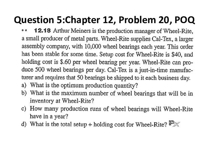
Question 5:Chapter 12, Problem 20, POQ
Question 5:Chapter 12, Problem 20, POQ
© Wiley 2010
Quantity Discount Model
Same as the EOQ model, except:
Unit price
© Wiley 2010
Quantity Discount Model
Same as the EOQ model, except:
Unit price
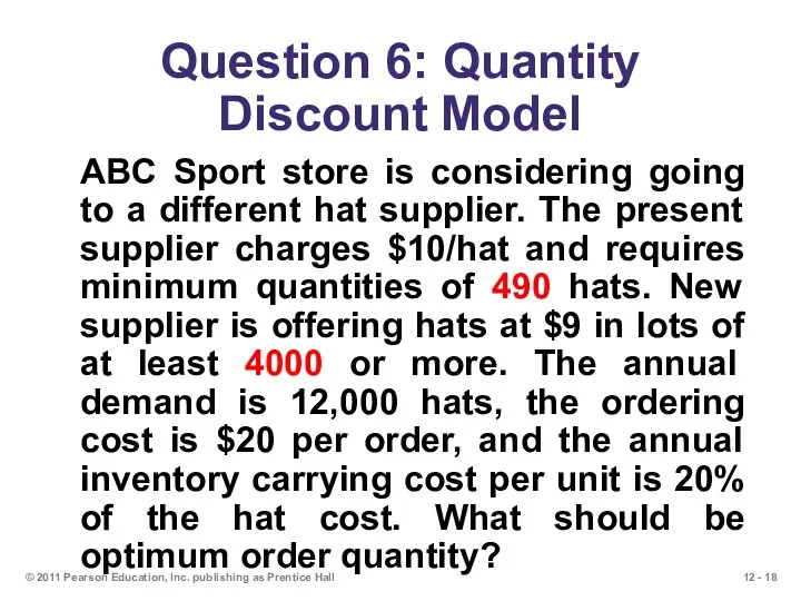
Question 6: Quantity Discount Model
ABC Sport store is considering going to
Question 6: Quantity Discount Model
ABC Sport store is considering going to
© 2011 Pearson Education, Inc. publishing as Prentice Hall
Holding Cost=
© 2011 Pearson Education, Inc. publishing as Prentice Hall
Holding Cost=
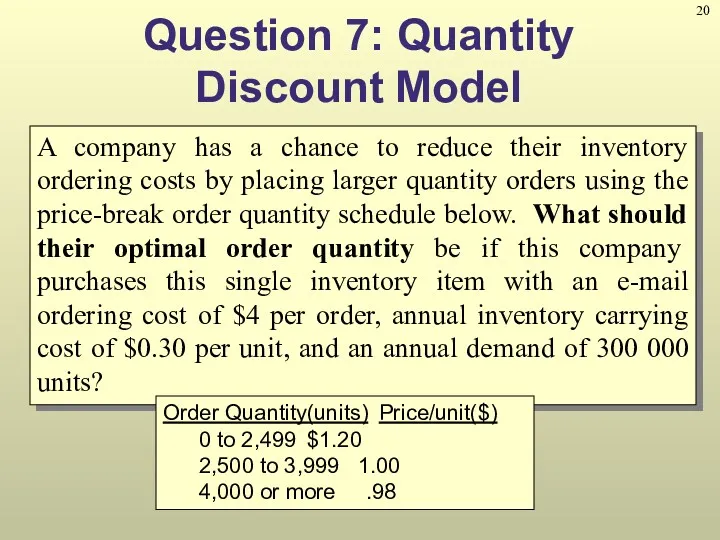
Question 7: Quantity Discount Model
A company has a chance to reduce
Question 7: Quantity Discount Model
A company has a chance to reduce
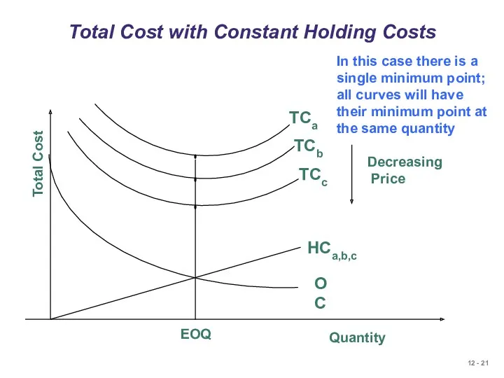
Total Cost with Constant Holding Costs
In this case there is
Total Cost with Constant Holding Costs
In this case there is
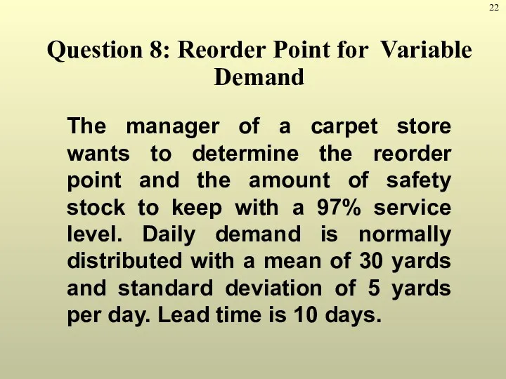
Question 8: Reorder Point for Variable Demand
The manager of a
Question 8: Reorder Point for Variable Demand
The manager of a
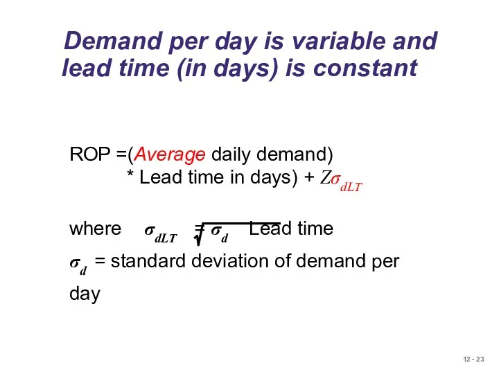
Demand per day is variable and lead time (in days)
Demand per day is variable and lead time (in days)
© 2011 Pearson Education, Inc. publishing as Prentice Hall
© 2011 Pearson Education, Inc. publishing as Prentice Hall
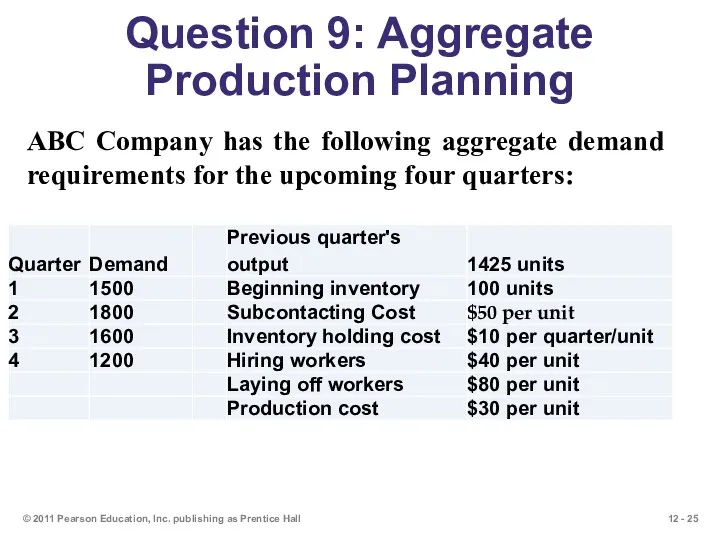
Question 9: Aggregate Production Planning
© 2011 Pearson Education, Inc. publishing as
Question 9: Aggregate Production Planning
© 2011 Pearson Education, Inc. publishing as
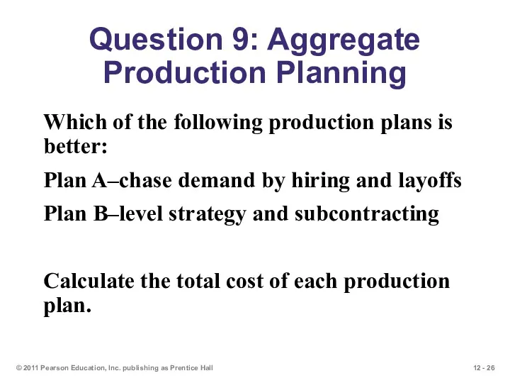
Question 9: Aggregate Production Planning
Which of the following production plans is
Question 9: Aggregate Production Planning
Which of the following production plans is
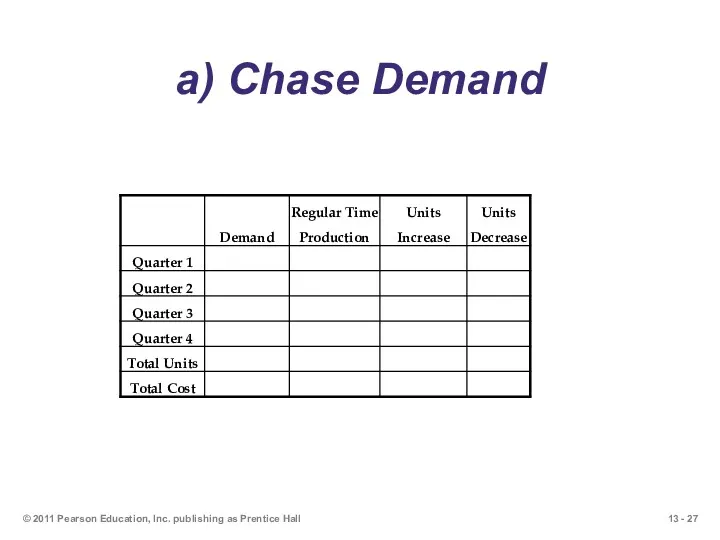
a) Chase Demand
© 2011 Pearson Education, Inc. publishing as Prentice Hall
a) Chase Demand
© 2011 Pearson Education, Inc. publishing as Prentice Hall
 Понятие и роль документационного обеспечения управления персоналом
 Программа рекомендаций. Referral program confidentia
 Стандарт управления проектами. Процессы управления проектом
 ВКР: Разработка прототипа информационной системы производственной логистики промышленного предприятия
 Современное делопроизводство. Документационное обеспечение управления
 Разработка мероприятий по развитию событийного туризма в Тульской области
 В поиске работы
 Управление человеческими ресурсами. Компетенция
 Организационная структура управления
 Диаграмма Парето
 Модели деловой карьеры
 Транспортно-экспедиционное обслуживание при международных автомобильных перевозках
 Использование процессного подхода как средства совершенствования системы управления организацией
 Модуль Управление персоналом (Нuman Resources). Управление организационными структурами
 Кейс-технологии
 Концепция Точно в срок
 Методологические основы менеджмента. Раздел 1
 Организация работы закусочной Блинная на 75 мест
 Zarządzanie agile
 Отчетная презентация СМС Санкт-Петербург-Балтийской дистанции пути за 3 квартал 2017 года
 Личность в системе управления
 Организационная структура управления проектом. Глава 4
 Управління якістю води у виробництві харчових продуктів. Лекції № 7-8
 Сущность и основные школы менеджмента
 Тема 2. Альтернативные логистические стратегии: проблема выбора
 Управление многоквартирным домом, управляющими организациями
 Баскет-метод
 Тайм-менджмент