- Risk Management

Содержание
- 2. Class #7 – Derivatives Pricing II 1 The binomial model 2 The Black –Scholes model 3
- 3. Class #7 – Derivatives Pricing II 1 The binomial model 2 The Black –Scholes model 3
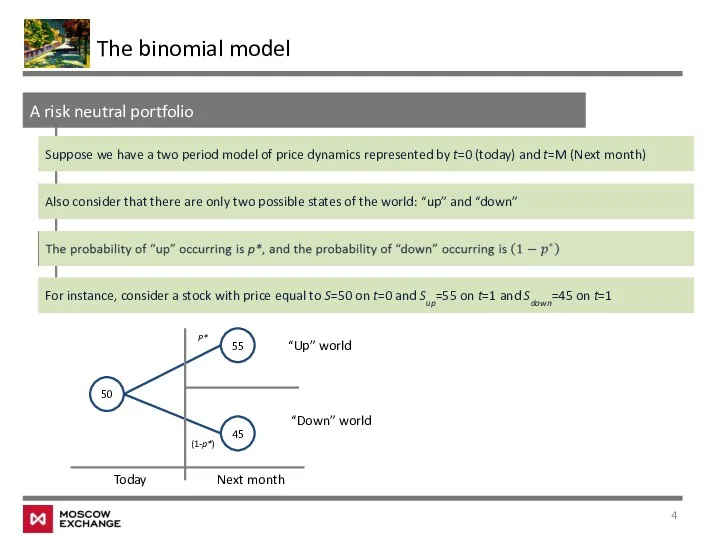
- 4. The binomial model A risk neutral portfolio Suppose we have a two period model of price
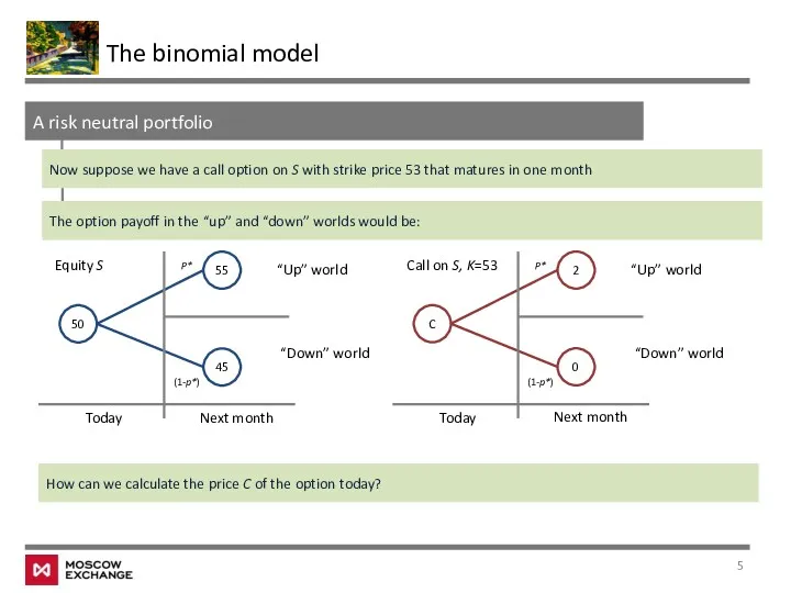
- 5. The binomial model A risk neutral portfolio Now suppose we have a call option on S
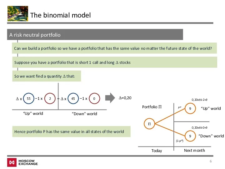
- 6. The binomial model A risk neutral portfolio Can we build a portfolio so we have a
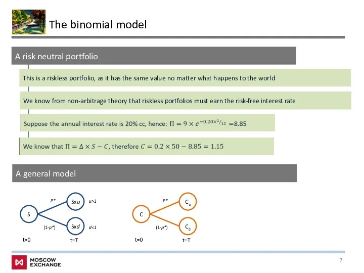
- 7. The binomial model A risk neutral portfolio This is a riskless portfolio, as it has the
- 8. The binomial model S Sxd t=0 P* (1-p*) Sxu t=T C Cd t=0 P* (1-p*) Cu
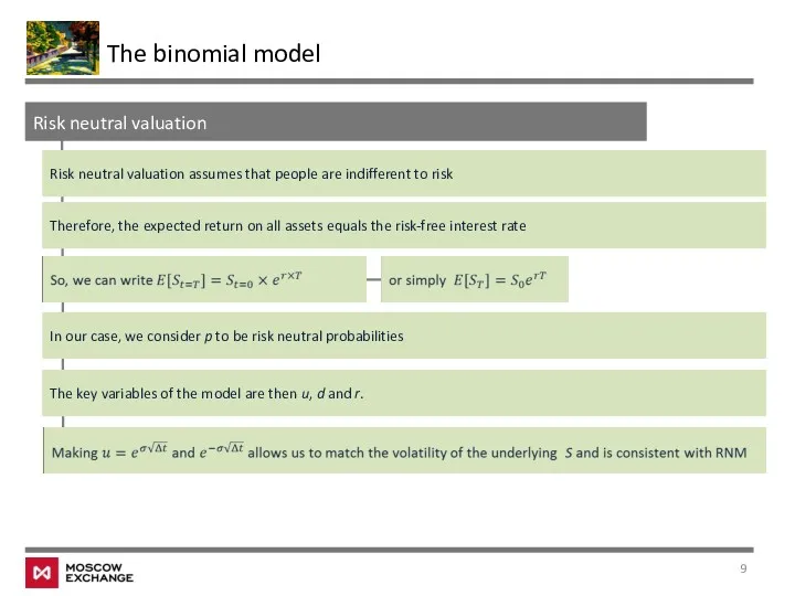
- 9. The binomial model Risk neutral valuation Risk neutral valuation assumes that people are indifferent to risk
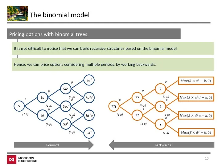
- 10. The binomial model Pricing options with binomial trees It is not difficult to notice that we
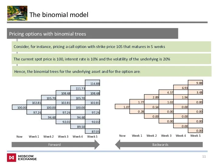
- 11. The binomial model Pricing options with binomial trees Consider, for instance, pricing a call option with
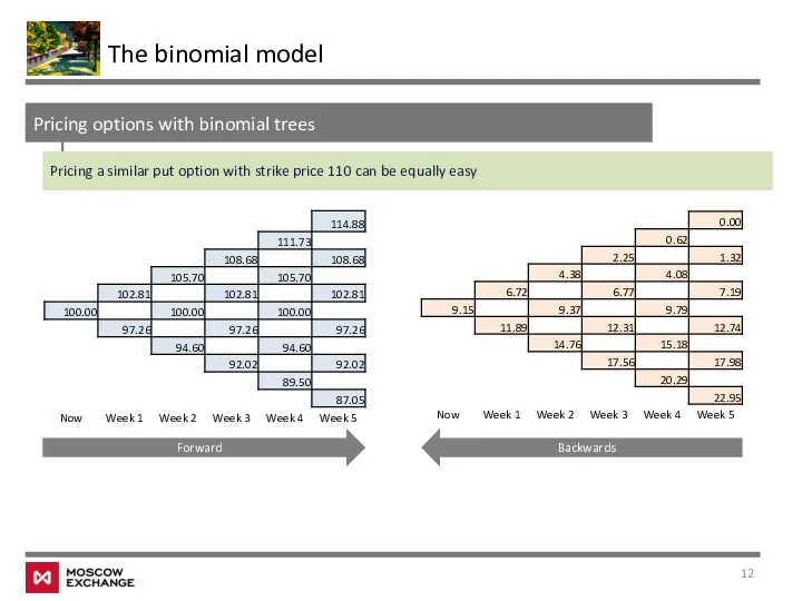
- 12. The binomial model Pricing options with binomial trees Pricing a similar put option with strike price
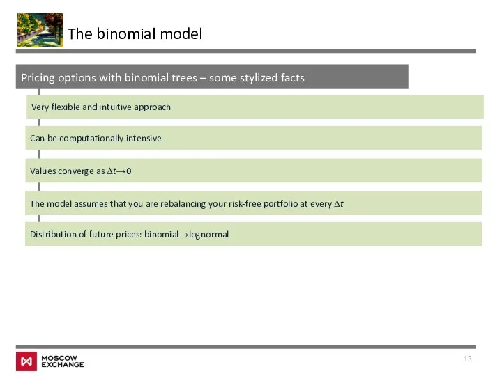
- 13. The binomial model Pricing options with binomial trees – some stylized facts Very flexible and intuitive
- 14. Class #7 – Derivatives Pricing II 1 The binomial model 2 The Black –Scholes model 3
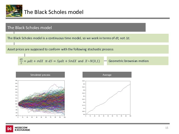
- 15. The Black Scholes model The Black Scholes model The Black Scholes model is a continuous time
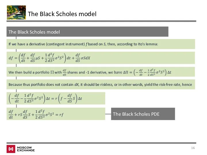
- 16. The Black Scholes model The Black Scholes model If we have a derivative (contingent instrument) f
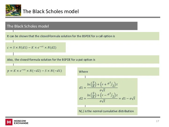
- 17. The Black Scholes model The Black Scholes model It can be shown that the closed-formula solution
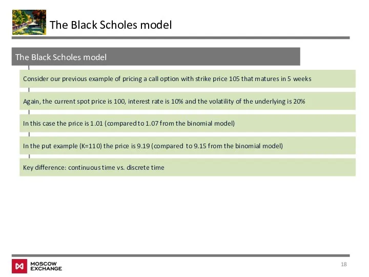
- 18. The Black Scholes model The Black Scholes model Consider our previous example of pricing a call
- 19. Hedging and the Greeks The Black Scholes model
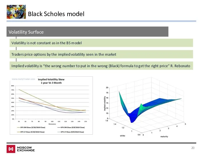
- 20. Black Scholes model Volatility Surface Implied volatility is “the wrong number to put in the wrong
- 21. Dynamic Delta hedging “In theory there is no difference between theory and practice. In practice there
- 22. Class #7 – Derivatives Pricing II 1 The binomial model 2 The Black –Scholes model 3
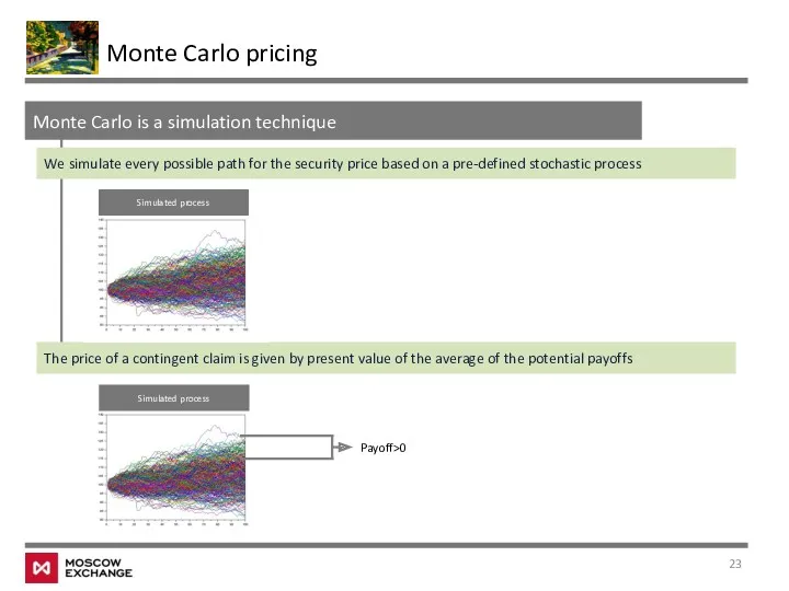
- 23. Monte Carlo is a simulation technique Monte Carlo pricing We simulate every possible path for the
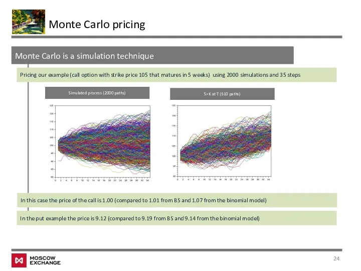
- 24. Monte Carlo is a simulation technique Monte Carlo pricing Pricing our example (call option with strike
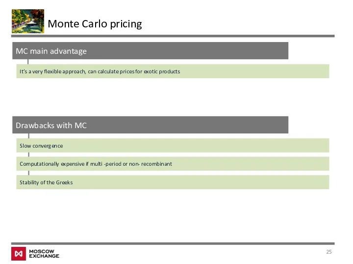
- 25. Drawbacks with MC Slow convergence Computationally expensive if multi -period or non- recombinant Stability of the
- 26. Class #7 – Derivatives Pricing II 1 The binomial model 2 The Black –Scholes model 3
- 27. Annex Useful References Options, Futures and Other Derivatives, John Hull, (2014); The Mathematics of Financial Derivatives
- 29. Скачать презентацию
Class #7 – Derivatives Pricing II
1
The binomial model
2
The Black –Scholes model
3
Monte
Class #7 – Derivatives Pricing II
1
The binomial model
2
The Black –Scholes model
3
Monte
Class #7 – Derivatives Pricing II
1
The binomial model
2
The Black –Scholes model
3
Monte
Class #7 – Derivatives Pricing II
1
The binomial model
2
The Black –Scholes model
3
Monte
The binomial model
A risk neutral portfolio
Suppose we have a two period
The binomial model
A risk neutral portfolio
Suppose we have a two period
The binomial model
A risk neutral portfolio
Now suppose we have a call
The binomial model
A risk neutral portfolio
Now suppose we have a call
The binomial model
A risk neutral portfolio
Can we build a portfolio so
The binomial model
A risk neutral portfolio
Can we build a portfolio so
The binomial model
A risk neutral portfolio
This is a riskless portfolio, as
The binomial model
A risk neutral portfolio
This is a riskless portfolio, as
The binomial model
S
Sxd
t=0
P*
(1-p*)
Sxu
t=T
C
Cd
t=0
P*
(1-p*)
Cu
t=T
u>1
d<1
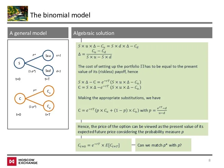
A general model
Algebraic solution
Hence, the price of the option
The binomial model
S
Sxd
t=0
P*
(1-p*)
Sxu
t=T
C
Cd
t=0
P*
(1-p*)
Cu
t=T
u>1
d<1
A general model
Algebraic solution
Hence, the price of the option
The binomial model
Risk neutral valuation
Risk neutral valuation assumes that people are
The binomial model
Risk neutral valuation
Risk neutral valuation assumes that people are
The binomial model
Pricing options with binomial trees
It is not difficult
The binomial model
Pricing options with binomial trees
It is not difficult
The binomial model
Pricing options with binomial trees
Consider, for instance, pricing
The binomial model
Pricing options with binomial trees
Consider, for instance, pricing
The binomial model
Pricing options with binomial trees
Pricing a similar put
The binomial model
Pricing options with binomial trees
Pricing a similar put
The binomial model
Pricing options with binomial trees – some stylized facts
Very
The binomial model
Pricing options with binomial trees – some stylized facts
Very
Class #7 – Derivatives Pricing II
1
The binomial model
2
The Black –Scholes model
3
Monte
Class #7 – Derivatives Pricing II
1
The binomial model
2
The Black –Scholes model
3
Monte
The Black Scholes model
The Black Scholes model
The Black Scholes model is
The Black Scholes model
The Black Scholes model
The Black Scholes model is
The Black Scholes model
The Black Scholes model
If we have a derivative
The Black Scholes model
The Black Scholes model
If we have a derivative
The Black Scholes model
The Black Scholes model
It can be shown that
The Black Scholes model
The Black Scholes model
It can be shown that
The Black Scholes model
The Black Scholes model
Consider our previous example of
The Black Scholes model
The Black Scholes model
Consider our previous example of
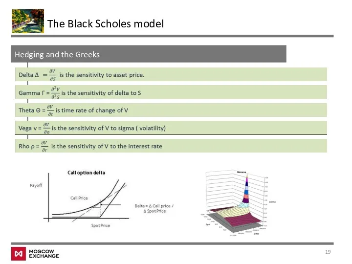
Hedging and the Greeks
The Black Scholes model
Hedging and the Greeks
The Black Scholes model
Black Scholes model
Volatility Surface
Implied volatility is “the wrong number to put
Black Scholes model
Volatility Surface
Implied volatility is “the wrong number to put
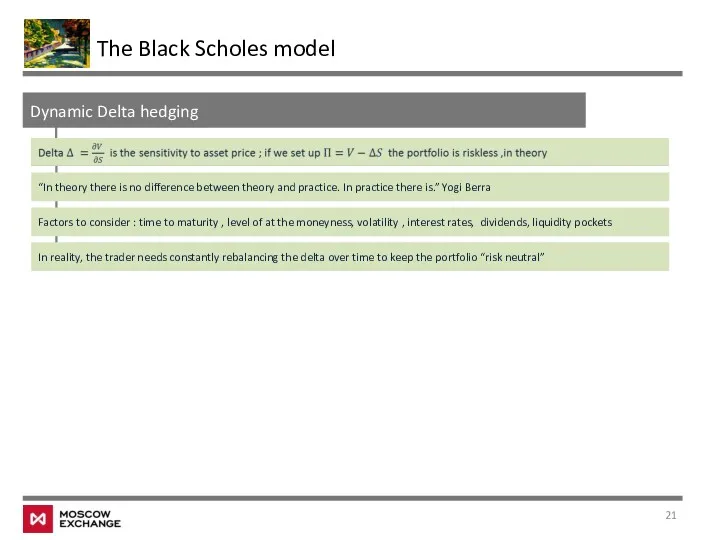
Dynamic Delta hedging
“In theory there is no difference between theory and
Dynamic Delta hedging
“In theory there is no difference between theory and
Class #7 – Derivatives Pricing II
1
The binomial model
2
The Black –Scholes model
3
Monte
Class #7 – Derivatives Pricing II
1
The binomial model
2
The Black –Scholes model
3
Monte
Monte Carlo is a simulation technique
Monte Carlo pricing
We simulate every
Monte Carlo is a simulation technique
Monte Carlo pricing
We simulate every
Monte Carlo is a simulation technique
Monte Carlo pricing
Pricing our example
Monte Carlo is a simulation technique
Monte Carlo pricing
Pricing our example
Drawbacks with MC
Slow convergence
Computationally expensive if multi -period or non- recombinant
Stability
Drawbacks with MC
Slow convergence
Computationally expensive if multi -period or non- recombinant
Stability
Class #7 – Derivatives Pricing II
1
The binomial model
2
The Black –Scholes model
3
Monte
Class #7 – Derivatives Pricing II
1
The binomial model
2
The Black –Scholes model
3
Monte
Annex
Useful References
Options, Futures and Other Derivatives, John Hull, (2014);
The Mathematics of
Annex
Useful References
Options, Futures and Other Derivatives, John Hull, (2014);
The Mathematics of
 Управление сбытом продукции в организации (на материалах ООО Ахтамар)
 Подбор персонала. Фриланс-рекрутинг
 Организация работы ресторана итальянской кухни на 150 мест
 Принятие управленческих решений
 Конкурс на присвоение звания Лучший по профессии молодой работник Октябрьской дирекции управления движением 2016
 Теория управления
 Обучение новых сотрудников
 Карта инструментов работы управляющего
 Управление затратами на качество
 Теория контрактов. Тема 4
 Выявление профессиональных компетенций инновационного менеджера
 Организация технического обслуживания производства
 Этика и этикет делового общения
 Бережливое производство. Учимся видеть потери
 Научные школы менеджмента
 Совершенствование кадровой политики государственного унитарного предприятия ГУП Водоканал Санкт-Петербурга
 Туристский комплекс как объект управления
 Организация электронного документооборота в компании
 Методы управления рисками
 Розробка стратегії антикризового менеджменту туристичного підприємства
 Понятие, содержание и значение делопроизводства
 Общественное мнение и управленческая деятельность (тема 15)
 Жизненный цикл проекта и продукта
 Оценка персонала компании
 Ситуационные центры: фокус кросс-отраслевых интересов
 Управление инновационными преобразованиями. Реинжиниринг и инновационные деловые процессы
 Обеспечение транспортно-логистических терминалов. Эксплуатация и автоматизация работы портов. Опасные грузы. (Тема 3)
 Разработка управленческих решений