- Analyzing a Case Study – CS #1. Acoustic

Содержание
- 2. Analyzing a Case Study – CS #1 Here are the steps when coming to analyze a
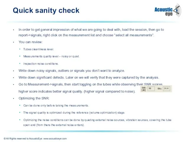
- 3. Quick sanity check In order to get general impression of what we are going to deal
- 4. Generate a visual reference The APR is a comparative method. Faults are detected by comparing a
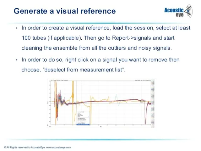
- 5. Generate a visual reference In order to create a visual reference, load the session, select at
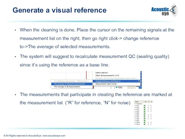
- 6. Generate a visual reference When the cleaning is done, Place the cursor on the remaining signals
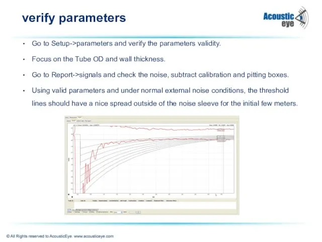
- 7. verify parameters Go to Setup->parameters and verify the parameters validity. Focus on the Tube OD and
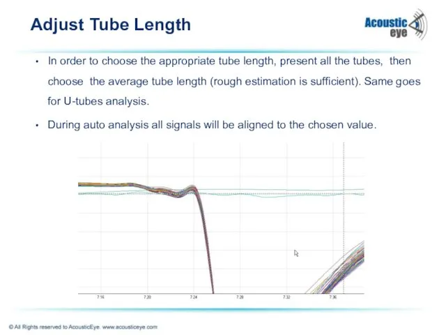
- 8. Adjust Tube Length In order to choose the appropriate tube length, present all the tubes, then
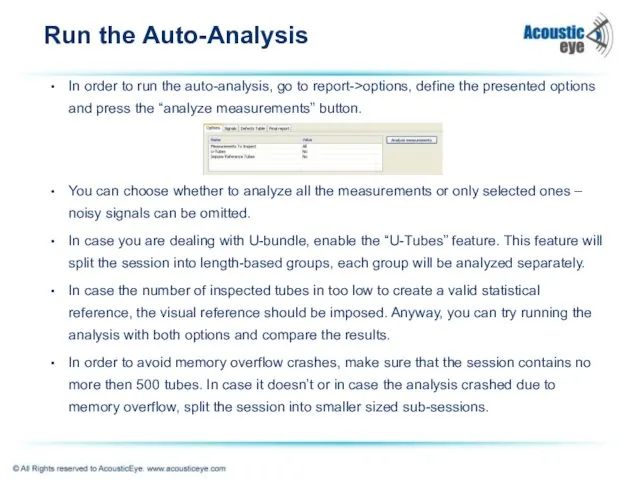
- 9. Run the Auto-Analysis In order to run the auto-analysis, go to report->options, define the presented options
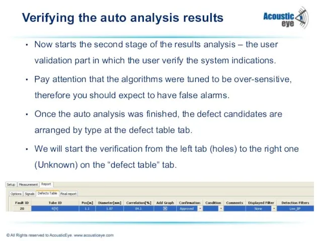
- 10. Verifying the auto analysis results Now starts the second stage of the results analysis – the
- 11. Verifying the auto analysis results Just by looking at the initial indications list we can learn
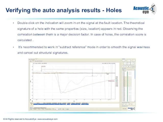
- 12. Verifying the auto analysis results - Holes Double click on the indication will zoom in on
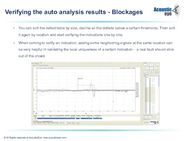
- 13. Verifying the auto analysis results - Blockages You can sort the defect table by size, decline
- 14. Verifying the auto analysis results - Erosions Those types of erosions were declined since they are
- 15. Verifying the auto analysis results - Pitting Checking the “history” of a signal helps validate the
- 16. Quick Full Manual Verification The final stage of the analysis is quick manual review of all
- 17. Miscellaneous – Filters Usage Different types of defects live in different frequency range. Blockages, Pitting and
- 18. Miscellaneous – Filters Usage Small Pitting Detection Using the “None” filter: Using the “high_bp” filter:
- 19. Miscellaneous – Differentiating Pitting and Erosions Differentiating between Pitting and Erosions can be done based on
- 21. Скачать презентацию
Analyzing a Case Study – CS #1
Here are the steps when
Analyzing a Case Study – CS #1
Here are the steps when
Quick sanity check
In order to get general impression of what we
Quick sanity check
In order to get general impression of what we
Generate a visual reference
The APR is a comparative method. Faults are
Generate a visual reference
The APR is a comparative method. Faults are
Generate a visual reference
In order to create a visual reference, load
Generate a visual reference
In order to create a visual reference, load
Generate a visual reference
When the cleaning is done, Place the cursor
Generate a visual reference
When the cleaning is done, Place the cursor
verify parameters
Go to Setup->parameters and verify the parameters validity.
Focus on the
verify parameters
Go to Setup->parameters and verify the parameters validity.
Focus on the
Adjust Tube Length
In order to choose the appropriate tube length, present
Adjust Tube Length
In order to choose the appropriate tube length, present
Run the Auto-Analysis
In order to run the auto-analysis, go to report->options,
Run the Auto-Analysis
In order to run the auto-analysis, go to report->options,
Verifying the auto analysis results
Now starts the second stage of the
Verifying the auto analysis results
Now starts the second stage of the
Verifying the auto analysis results
Just by looking at the initial indications
Verifying the auto analysis results
Just by looking at the initial indications
Verifying the auto analysis results - Holes
Double click on the indication
Verifying the auto analysis results - Holes
Double click on the indication
Verifying the auto analysis results - Blockages
You can sort the defect
Verifying the auto analysis results - Blockages
You can sort the defect
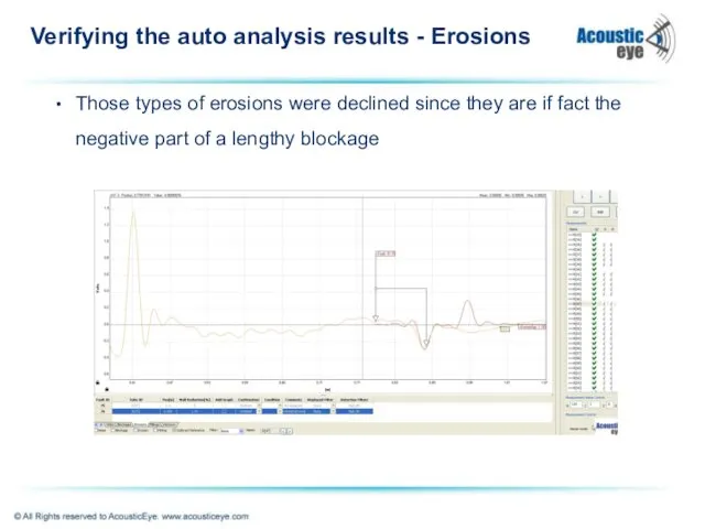
Verifying the auto analysis results - Erosions
Those types of erosions were
Verifying the auto analysis results - Erosions
Those types of erosions were
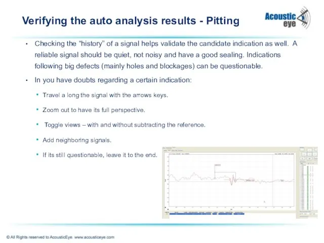
Verifying the auto analysis results - Pitting
Checking the “history” of a
Verifying the auto analysis results - Pitting
Checking the “history” of a
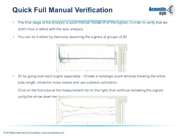
Quick Full Manual Verification
The final stage of the analysis is quick
Quick Full Manual Verification
The final stage of the analysis is quick
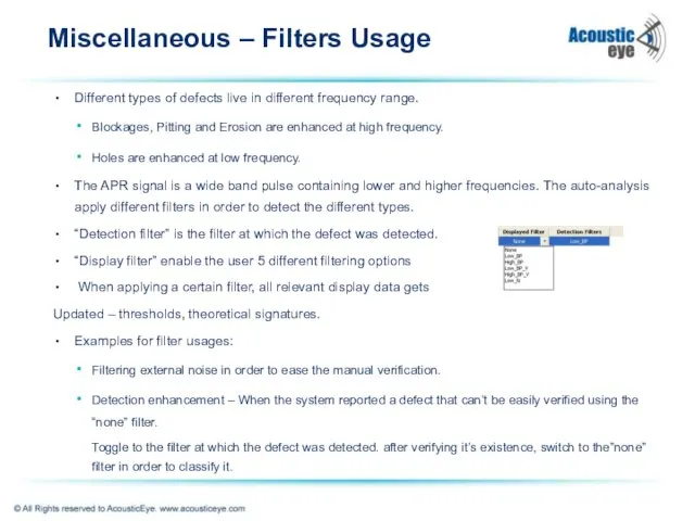
Miscellaneous – Filters Usage
Different types of defects live in different frequency
Miscellaneous – Filters Usage
Different types of defects live in different frequency
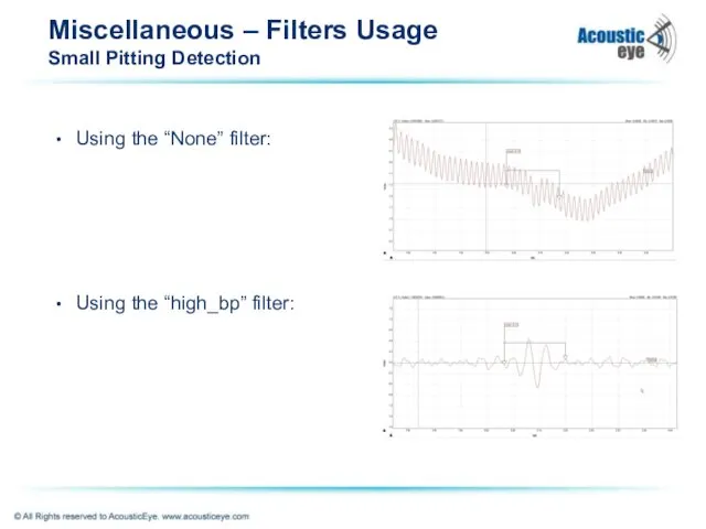
Miscellaneous – Filters Usage
Small Pitting Detection
Using the “None” filter:
Using the “high_bp”
Miscellaneous – Filters Usage
Small Pitting Detection
Using the “None” filter:
Using the “high_bp”
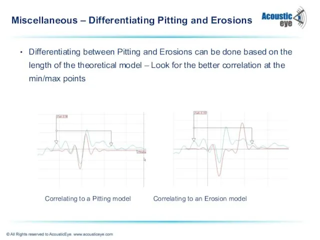
Miscellaneous – Differentiating Pitting and Erosions
Differentiating between Pitting and Erosions can
Miscellaneous – Differentiating Pitting and Erosions
Differentiating between Pitting and Erosions can
 Презентация Детская организация РОСТ
 Балеринки из бумаги - чудесное украшение к Новому году. Диск
 Двигательная активность
 Организационные формы обучения
 психологические особенности детей 7 лет
 Индийский океан
 портфолио учителя-логопеда Бакиной Ольги Нколаевны
 cad-08a6b4b6
 Список приёмов при выполнении домашних заданий.
 Презентация Гимн,герб, флаг
 Основы религиозных культур и светской этики
 Межгосударственные отношения. Внешние функции государства
 Q Тобина (1)
 S7 Airlines
 Дорохов Михаил 9А Искусственный биоценоз
 Электрические характеристики антенн. Лекция 2
 Охрана труда при работе с компьютерной техникой
 Общественная организация Союз пионерских организаций Нижегородской области
 Методика логопедического восстановления голоса у детей
 Класcный час СНГ
 Жаңа дәуір философиясындағы сенсуалистік және рационалистік таным теорияларыны әлеуметтік-философиялық негіздері ретінде
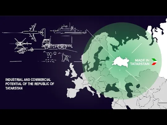 Industrial and commercial potential of the republic
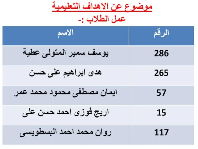 موضوع عن االهداف التعليمية
 Презентация к уроку Реакции ионного обмена (8 кл)
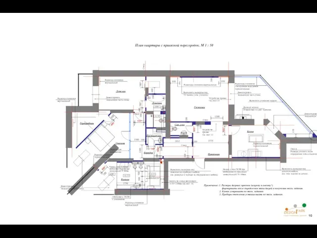 План квартиры с привязкой перегородок
 Машиностроение. Структура машиностроения
 крылатые выражения из романа Евгений Онегин
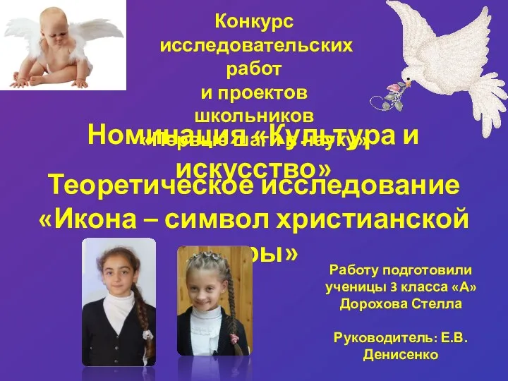 Икона – символ христианской веры