- Fast Frequency and Response Measurements using FFTs

Содержание
- 2. Accurately Detect a Tone What is the exact frequency and amplitude of a tone embedded in
- 3. Presentation Overview Why use the frequency domain? FFT – a short introduction Frequency interpolation Improvements using
- 4. Clean Single Tone Measurement Clean sine tone Easy to measure Clean tone spectrum
- 5. Noisy Tone Measurement Noisy signal Difficult to measure in the time domain Noisy signal spectrum Easier
- 6. Fast Fourier Transform (FFT) Fundamentals (Ideal Case) The tone frequency is an exact multiple of the
- 7. FFT Fundamentals (Realistic Case) The tone frequency is not a multiple of the frequency resolution
- 8. Input Frequency Hits Exactly a Bin Only one bin is activated
- 9. Input Frequency is +0.01 Bin “off” More bins are activated
- 10. Input Frequency is +0.25 Bin “off”
- 11. Input Frequency is +0.50 Bin “off” Highest side-lobes
- 12. Input Frequency is +0.75 Bin “off” The Side lobe levels decrease
- 13. Input Frequency is +1.00 Bin “off” Only one bin is activated
- 14. The Envelope Function
- 15. The Mathematics Envelope function: Bin offset: Real amplitude:
- 16. Demo Amplitude and frequency detection by Sin(x) / x interpolation
- 17. Aliasing of the Side-Lobes
- 18. Weighted Measurement Apply a Window to the signal
- 19. Weighted Spectrum Measurement Apply a Window to the Signal 20 -60 -40 -20 0 25 0
- 20. Rectangular and Hanning Windows Side lobes for Hanning Window are significantly lower than for Rectangular window
- 21. Input Frequency Exactly Hits a Bin Three bins are activated
- 22. Input Frequency is +0.25 Bin “off” More bins are activated
- 23. Input Frequency is +0.50 Bin “off” Highest side-lobes
- 24. Input Frequency is +0.75 Bin “off” The Side lobe levels decrease
- 25. Input Frequency is +1.00 Bin “off” Only three bins activated
- 26. The Mathematics for Hanning ... Envelope: Bin Offset: Amplitude:
- 27. A LabVIEW Tool Tone detector LabVIEW virtual instrument (VI)
- 28. Demo Amplitude and frequency detection using a Hanning Window (named after Von Hann) Real world demo
- 29. Frequency Detection Resolution
- 30. Amplitude Detection Resolution
- 31. Phase Detection Resolution
- 32. Conclusions Traditional counters resolve 10 digits in one second FFT techniques can do this in much
- 34. Скачать презентацию
Accurately Detect a Tone
What is the exact frequency and amplitude
Accurately Detect a Tone
What is the exact frequency and amplitude
Presentation Overview
Why use the frequency domain?
FFT – a short introduction
Frequency interpolation
Improvements
Presentation Overview
Why use the frequency domain?
FFT – a short introduction
Frequency interpolation
Improvements
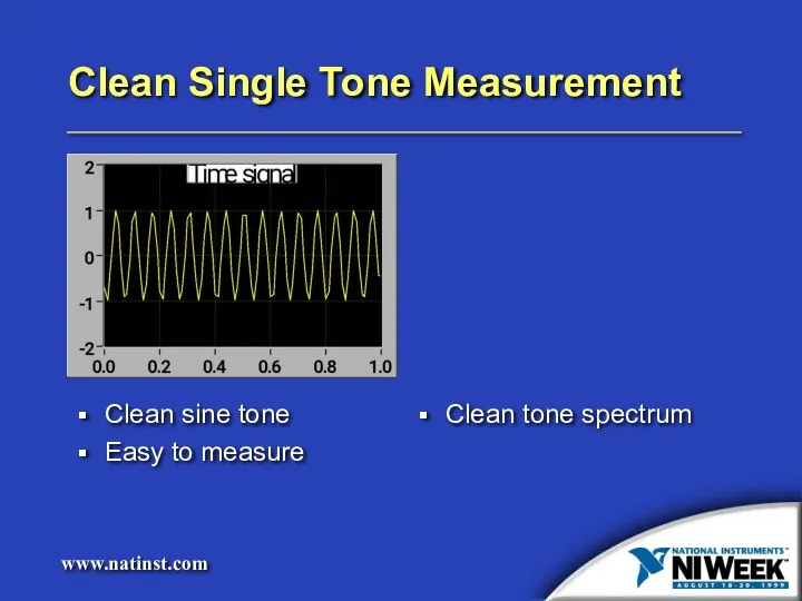
Clean Single Tone Measurement
Clean sine tone
Easy to measure
Clean tone spectrum
Clean Single Tone Measurement
Clean sine tone
Easy to measure
Clean tone spectrum
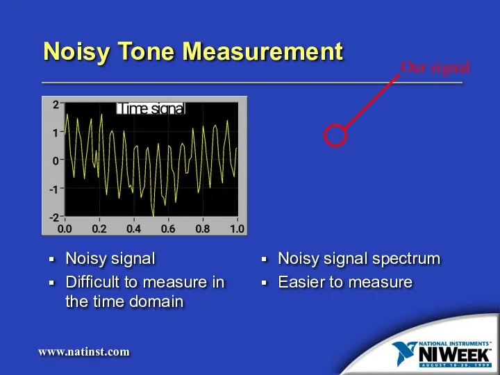
Noisy Tone Measurement
Noisy signal
Difficult to measure in the time domain
Noisy signal
Noisy Tone Measurement
Noisy signal
Difficult to measure in the time domain
Noisy signal
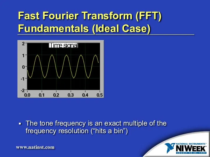
Fast Fourier Transform (FFT) Fundamentals (Ideal Case)
The tone frequency is an
Fast Fourier Transform (FFT) Fundamentals (Ideal Case)
The tone frequency is an
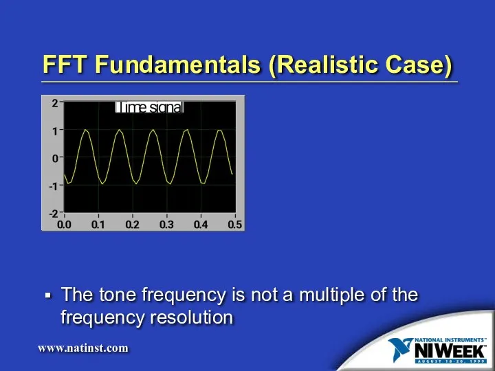
FFT Fundamentals (Realistic Case)
The tone frequency is not a multiple of
FFT Fundamentals (Realistic Case)
The tone frequency is not a multiple of
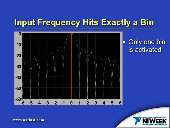
Input Frequency Hits Exactly a Bin
Only one bin is activated
Input Frequency Hits Exactly a Bin
Only one bin is activated
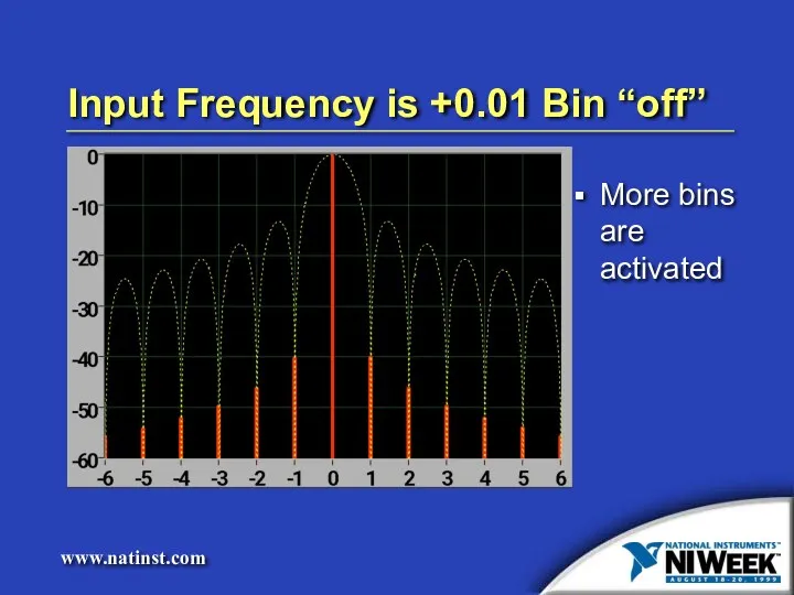
Input Frequency is +0.01 Bin “off”
More bins are activated
Input Frequency is +0.01 Bin “off”
More bins are activated
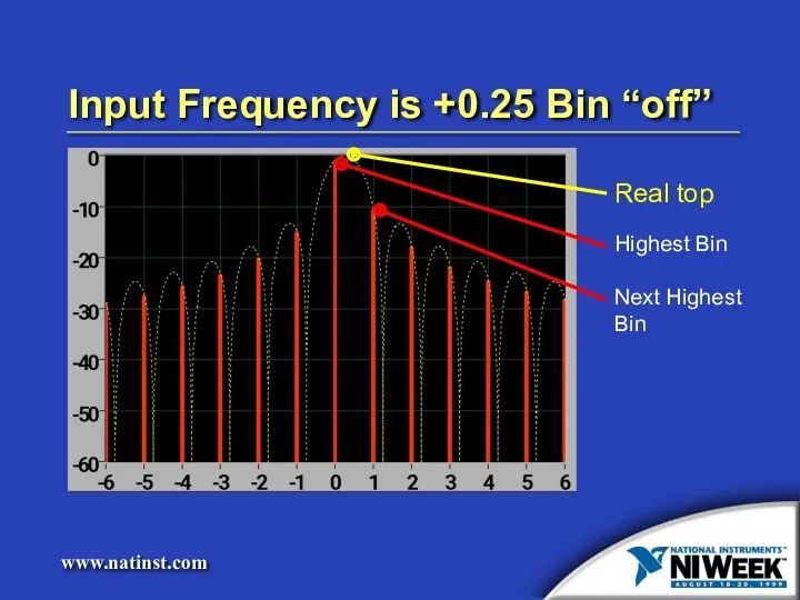
Input Frequency is +0.25 Bin “off”
Input Frequency is +0.25 Bin “off”
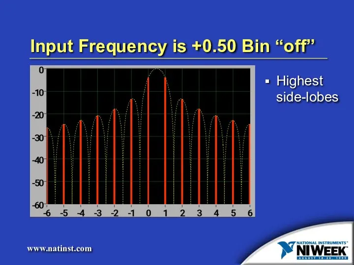
Input Frequency is +0.50 Bin “off”
Highest side-lobes
Input Frequency is +0.50 Bin “off”
Highest side-lobes
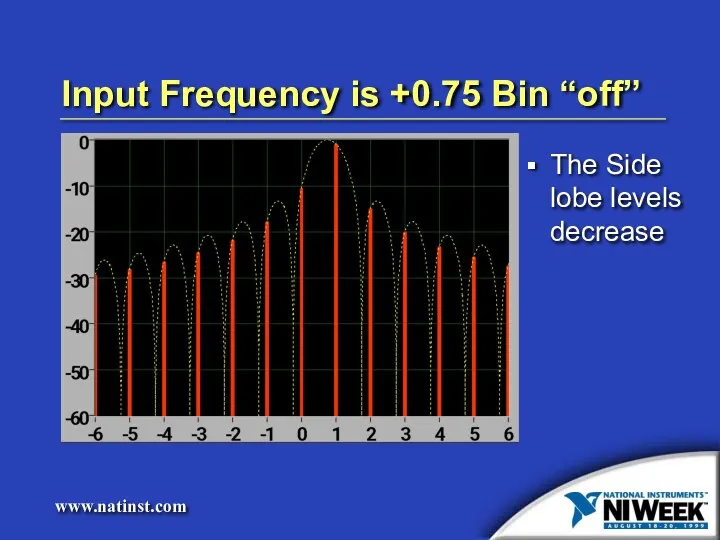
Input Frequency is +0.75 Bin “off”
The Side lobe levels decrease
Input Frequency is +0.75 Bin “off”
The Side lobe levels decrease
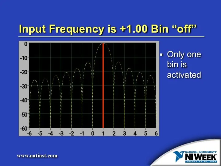
Input Frequency is +1.00 Bin “off”
Only one bin is activated
Input Frequency is +1.00 Bin “off”
Only one bin is activated
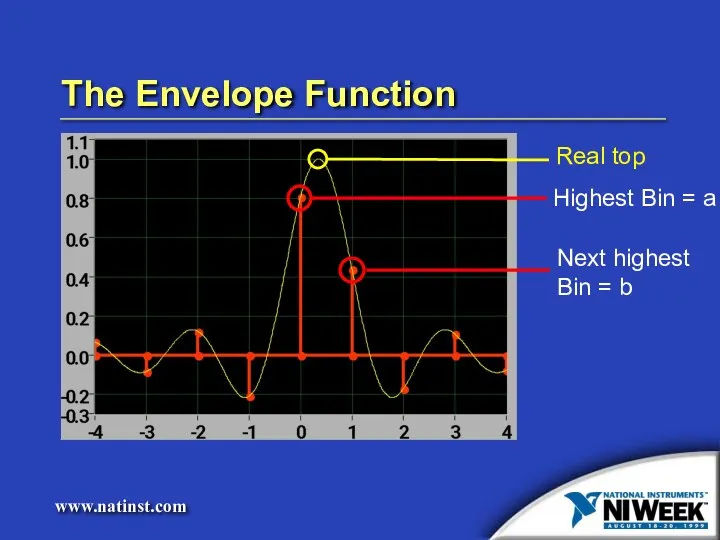
The Envelope Function
The Envelope Function
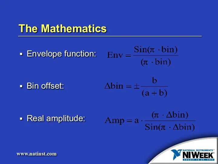
The Mathematics
Envelope function:
Bin offset:
Real amplitude:
The Mathematics
Envelope function:
Bin offset:
Real amplitude:
Demo
Amplitude and frequency detection by Sin(x) / x interpolation
Demo
Amplitude and frequency detection by Sin(x) / x interpolation
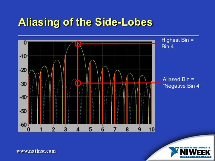
Aliasing of the Side-Lobes
Aliasing of the Side-Lobes
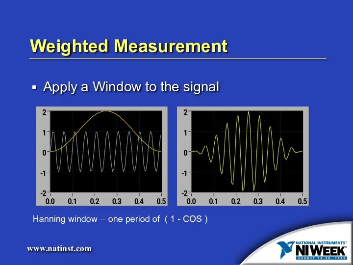
Weighted Measurement
Apply a Window to the signal
Weighted Measurement
Apply a Window to the signal
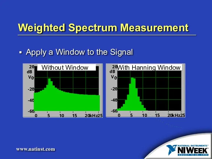
Weighted Spectrum Measurement
Apply a Window to the Signal
20
-60
-40
-20
0
25
0
5
10
15
20
Without Window
kHz
dBV
20
-60
-40
-20
0
25
0
5
10
15
20
With Hanning Window
kHz
dBV
Weighted Spectrum Measurement
Apply a Window to the Signal
20
-60
-40
-20
0
25
0
5
10
15
20
Without Window
kHz
dBV
20
-60
-40
-20
0
25
0
5
10
15
20
With Hanning Window
kHz
dBV

Rectangular and Hanning Windows
Side lobes for Hanning Window are significantly lower
Rectangular and Hanning Windows
Side lobes for Hanning Window are significantly lower
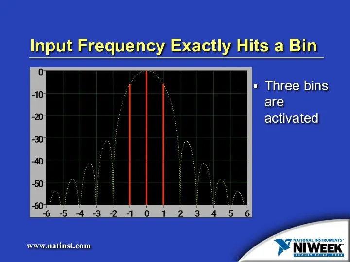
Input Frequency Exactly Hits a Bin
Three bins are activated
Input Frequency Exactly Hits a Bin
Three bins are activated

Input Frequency is +0.25 Bin “off”
More bins are activated
Input Frequency is +0.25 Bin “off”
More bins are activated

Input Frequency is +0.50 Bin “off”
Highest side-lobes
Input Frequency is +0.50 Bin “off”
Highest side-lobes
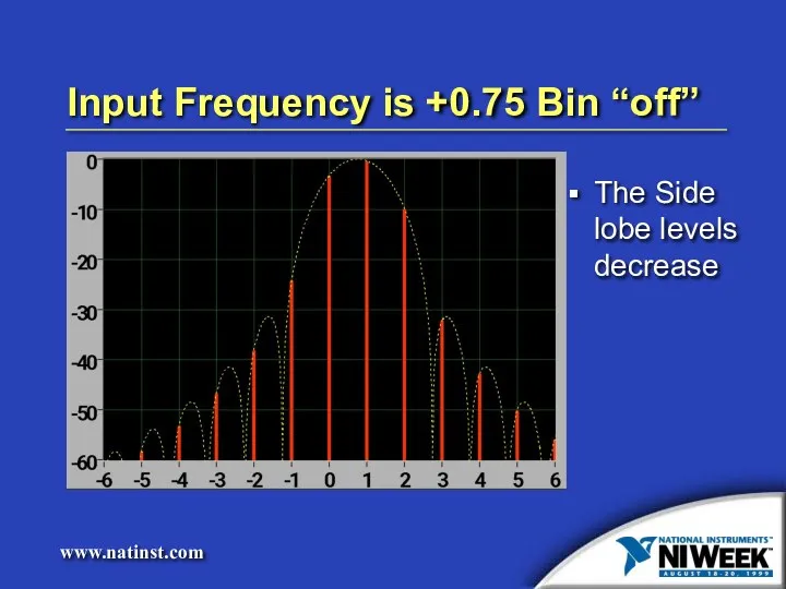
Input Frequency is +0.75 Bin “off”
The Side lobe levels decrease
Input Frequency is +0.75 Bin “off”
The Side lobe levels decrease
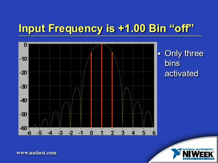
Input Frequency is +1.00 Bin “off”
Only three bins activated
Input Frequency is +1.00 Bin “off”
Only three bins activated
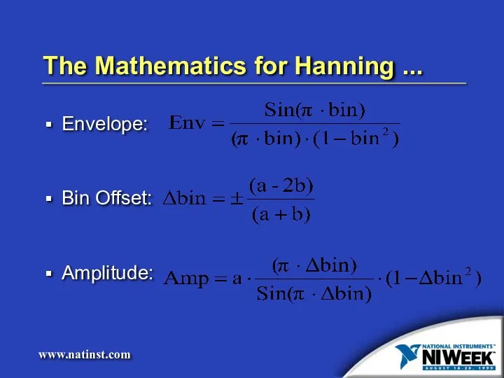
The Mathematics for Hanning ...
Envelope:
Bin Offset:
Amplitude:
The Mathematics for Hanning ...
Envelope:
Bin Offset:
Amplitude:
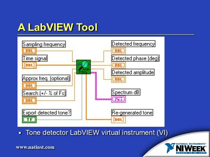
A LabVIEW Tool
Tone detector LabVIEW virtual instrument (VI)
A LabVIEW Tool
Tone detector LabVIEW virtual instrument (VI)
Demo
Amplitude and frequency detection using a Hanning Window (named after Von
Demo
Amplitude and frequency detection using a Hanning Window (named after Von
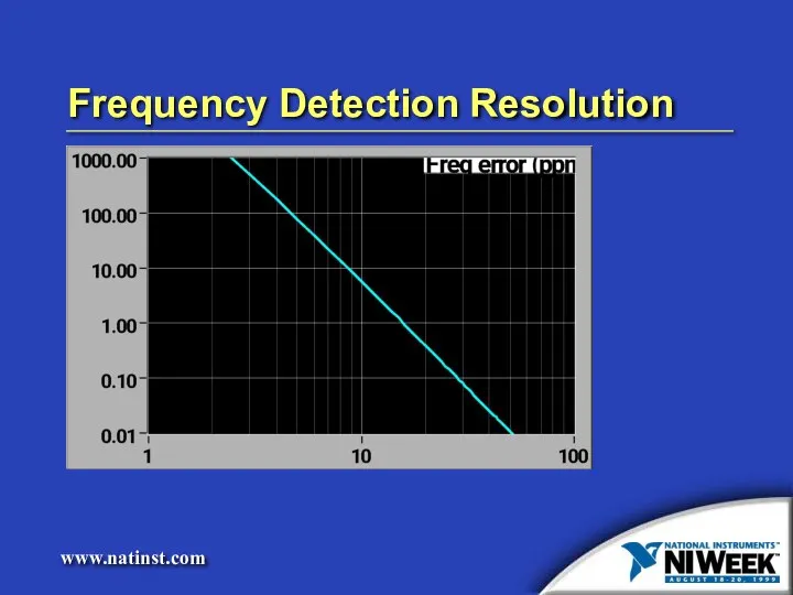
Frequency Detection Resolution
Frequency Detection Resolution

Amplitude Detection Resolution
Amplitude Detection Resolution
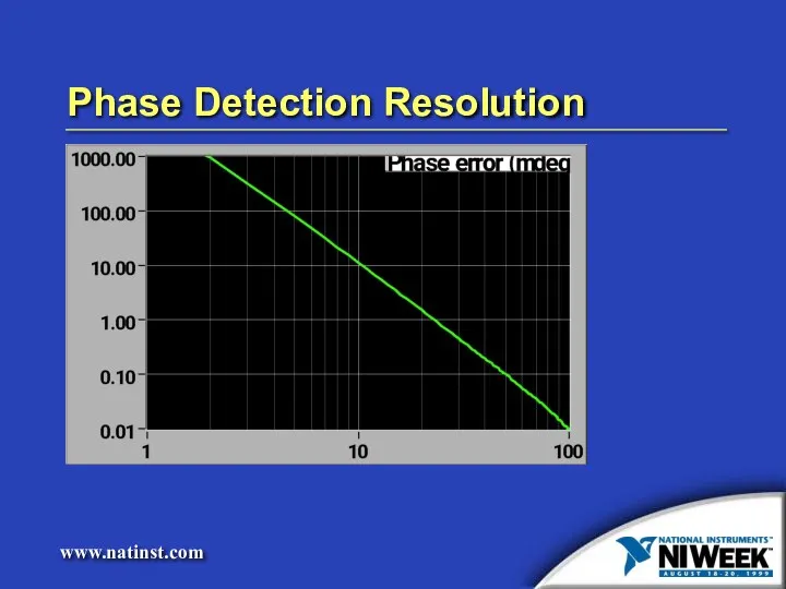
Phase Detection Resolution
Phase Detection Resolution
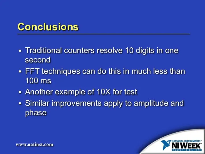
Conclusions
Traditional counters resolve 10 digits in one second
FFT techniques can do
Conclusions
Traditional counters resolve 10 digits in one second
FFT techniques can do
 классный час Широкая Масленица: обычаи и обряды
 Мой любимый детский сад. Экскурсия в медицинский кабинет
 презентация к статье Преемственность урочной и внеурочной деятельности – единая система достижения планируемых результатов.
 Обобщающий урок по теме Все действия с рациональными числами 6 класс
 Завод имени Кузнецова. Испытательная площадка
 Aparate de fotografiat. Fotografia digitală
 Защита и автоматика ЛЭП
 Нашей дорогой, любимой маме и бабушке, посвящается
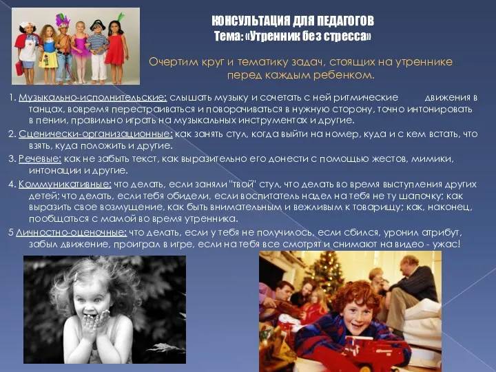 Консультация для воспитателей Утренник без стресса
 Воздушное питание растений. Фотосинтез
 Презентация по картине И.И. Шишкина Зима
 Песня Мы вместе
 Пищевые отравления
 Шутливый жанр
 Причины возникновения речевых нарушений у детей
 Современные модели образовательного процесса ДОУ
 Методы сбора и обработки данных при помощи Python. Урок 5
 Административная ответственность физических и юридических лиц. Субъекты ответственности за нарушения таможенных правил
 Прохідницький комбайн
 Современное состояние и охрана атмосферы
 Экологическая обстановка Санкт-Петербурга
 Социальные проблемы валютного ипотечного кредитования в России и пути их решения
 Влияние параметров режимов сварки на качество сварного шва
 Проект: Мир профессий - АТЕЛЬЕ
 Презентация классного часа Перед лицом возможной опасности
 Визуализация. Повышение наглядности материала
 Анализ повреждений магистралей первичной сети и разработка мероприятий по сокращению времени проведения ремонтных работ
 Гемодинамика. Движение крови по сосудам