- Intro to machine learning

Содержание
- 2. Recap What is linear regression? Why study linear regression? What can we use it for? How
- 3. Objectives Extension of linear regressions Interaction Polynomial Classification Logistic Regression Confusion Metric
- 4. Potential Problems with Linear Regression
- 5. Linear Models Linear models are relatively simple to describe and implement They have advantages over other
- 6. Then why do we need extensions? Linear regression makes some assumptions that are easily violated in
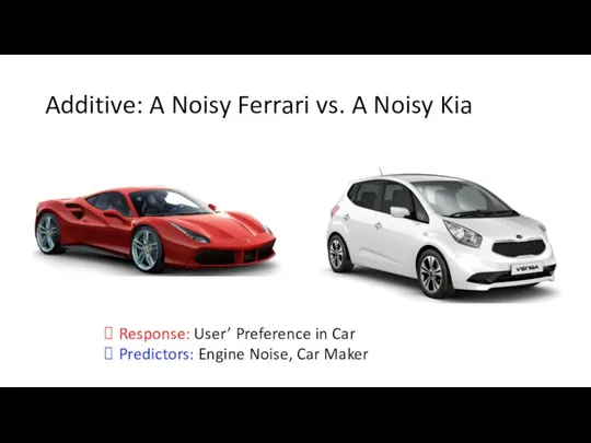
- 7. Additive: A Noisy Ferrari vs. A Noisy Kia Response: User’ Preference in Car Predictors: Engine Noise,
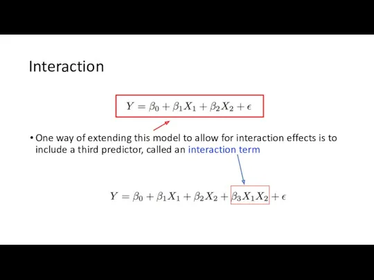
- 8. Interaction One way of extending this model to allow for interaction effects is to include a
- 9. Finding Interaction Terms Domain Knowledge Automatic search over all possible combinations
- 10. Example – Interaction between TV and Radio A linear regression fit to sales using TV and
- 11. Example – Interaction between TV and Radio A linear regression fit to sales using TV and
- 12. Example (2) This suggests some synergy or interaction between the two predictors.
- 13. Example (3) After including the interaction term We can interpret β3 as the increase in the
- 14. Interactions Hierarchical Principle If we include an interaction term in our model, we should also include
- 15. Interaction between quantitative and qualitative variables -1
- 16. Interaction between quantitative and qualitative variables -2
- 17. Non-linearity (1)
- 18. Non-linearity (2)
- 19. Non-linearity (3)
- 20. In General Standard Linear Model Extend linear regression to settings in which the relationship between the
- 21. Polynomial Regression (1) The Auto data set. For a number of cars, mpg and horsepower are
- 22. Polynomial Regression (2) It is still a Linear Model
- 23. Classification Response variable is discrete or qualitative eye color∈{brown, blue, green} email∈ {spam, ham} expression ∈
- 24. Linear vs. Non-linear A Classification Example in 2-Dimensions, with Three different Flexibility Levels (a) (b) (C)
- 25. Example The annual incomes and monthly credit card balances of a number of individuals. The individuals
- 26. What if we treat the problem as follows? Instead of coding the qualitative response and estimating
- 27. Now, Can we use Linear Regression?
- 28. This is what we want
- 29. Logistic Regression (1)
- 30. Logistic Regression (2)
- 31. Parameter Estimation We need a loss function
- 32. Logistic Regression Cost Function (1)
- 33. Logistic Regression Cost Function (2) Thus we need a different Loss function
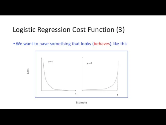
- 34. Logistic Regression Cost Function (3) We want to have something that looks (behaves) like this
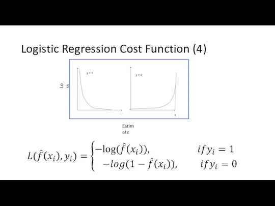
- 35. Logistic Regression Cost Function (4)
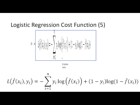
- 36. Logistic Regression Cost Function (5)
- 37. Parameter Estimation Now that we have the cost function, how should we use it to estimate
- 38. Doing Logistic Regression for Our Example
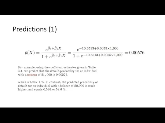
- 39. Predictions (1) For example, using the coefficient estimates given in Table 4.1, we predict that the
- 40. Predictions (2)
- 41. Multiple Logistic Regression
- 42. Interpreting the results of Logistic Regression
- 43. So How to Interpret the Results? Odds Log-Odds
- 44. Interpreting the results of Logistic Regression
- 45. Multiclass Classification (1) One versus All One versus One
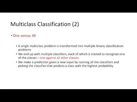
- 46. Multiclass Classification (2) One versus All A single multiclass problem is transformed into multiple binary classification
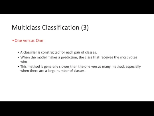
- 47. Multiclass Classification (3) One versus One A classifier is constructed for each pair of classes. When
- 48. Classification Metric
- 49. When Accuracy is Not Good Enough?
- 50. Some Simple Requirements for Good Classifier Better than average classifier Better than majority classifier
- 51. An Example Where We Need More than Just Accuracy – Recall and Precision
- 52. Confusion Matrix Binary Response (Yes/No) True positive: A positive sample correctly classified False positive: A negative
- 53. Precision (1) Fraction of positive predictions that are actually positive
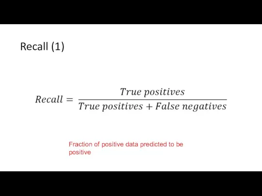
- 54. Recall (1) Fraction of positive data predicted to be positive
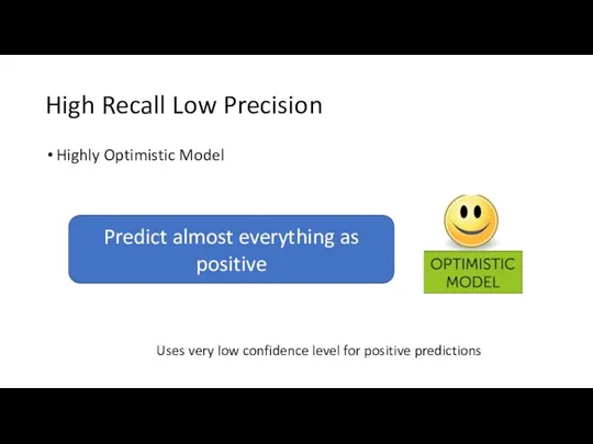
- 55. High Recall Low Precision Highly Optimistic Model Predict almost everything as positive Uses very low confidence
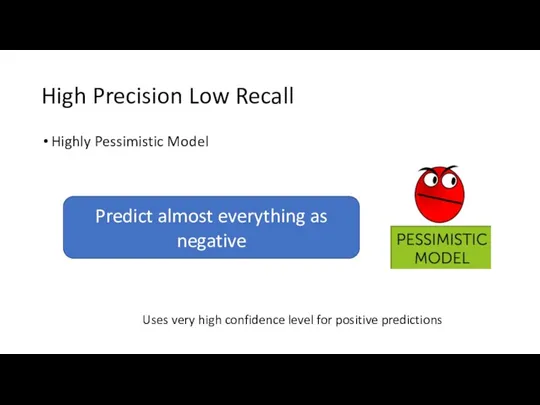
- 56. High Precision Low Recall Highly Pessimistic Model Predict almost everything as negative Uses very high confidence
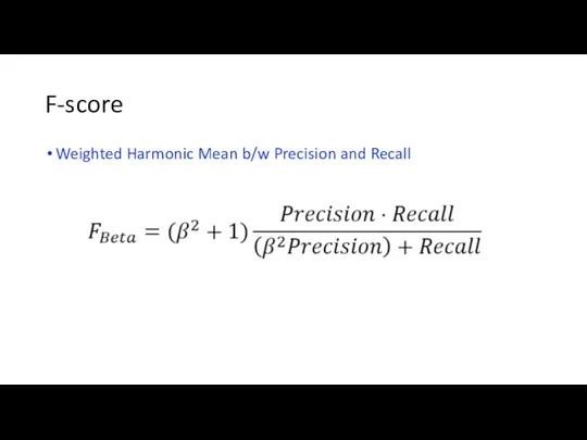
- 57. F-score Weighted Harmonic Mean b/w Precision and Recall
- 59. Скачать презентацию
Recap
What is linear regression?
Why study linear regression?
What can we use it
Recap
What is linear regression?
Why study linear regression?
What can we use it
Objectives
Extension of linear regressions
Interaction
Polynomial
Classification
Logistic Regression
Confusion Metric
Objectives
Extension of linear regressions
Interaction
Polynomial
Classification
Logistic Regression
Confusion Metric
Potential Problems with Linear Regression
Potential Problems with Linear Regression
Linear Models
Linear models are relatively simple to describe and implement
They have
Linear Models
Linear models are relatively simple to describe and implement
They have
Then why do we need extensions?
Linear regression makes some assumptions that
Then why do we need extensions?
Linear regression makes some assumptions that
Additive: A Noisy Ferrari vs. A Noisy Kia
Response: User’ Preference in
Additive: A Noisy Ferrari vs. A Noisy Kia
Response: User’ Preference in
Interaction
One way of extending this model to allow for interaction effects
Interaction
One way of extending this model to allow for interaction effects
Finding Interaction Terms
Domain Knowledge
Automatic search over all possible combinations
Finding Interaction Terms
Domain Knowledge
Automatic search over all possible combinations
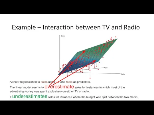
Example – Interaction between TV and Radio
A linear regression fit to
Example – Interaction between TV and Radio
A linear regression fit to
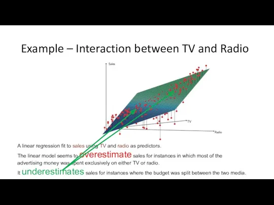
Example – Interaction between TV and Radio
A linear regression fit to
Example – Interaction between TV and Radio
A linear regression fit to
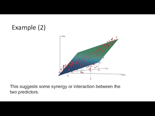
Example (2)
This suggests some synergy or interaction between the two predictors.
Example (2)
This suggests some synergy or interaction between the two predictors.
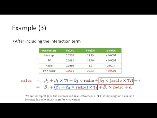
Example (3)
After including the interaction term
We can interpret β3 as the
Example (3)
After including the interaction term
We can interpret β3 as the
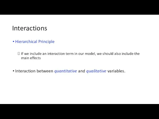
Interactions
Hierarchical Principle
If we include an interaction term in our model, we
Interactions
Hierarchical Principle
If we include an interaction term in our model, we
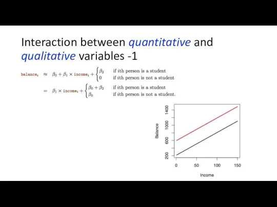
Interaction between quantitative and qualitative variables -1
Interaction between quantitative and qualitative variables -1
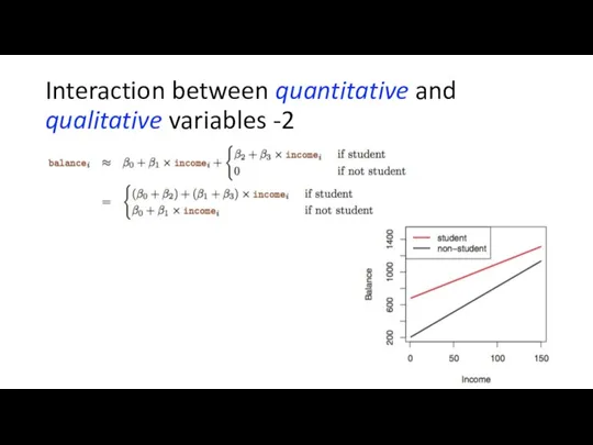
Interaction between quantitative and qualitative variables -2
Interaction between quantitative and qualitative variables -2
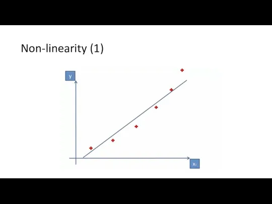
Non-linearity (1)
Non-linearity (1)
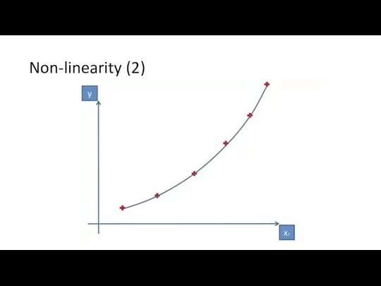
Non-linearity (2)
Non-linearity (2)
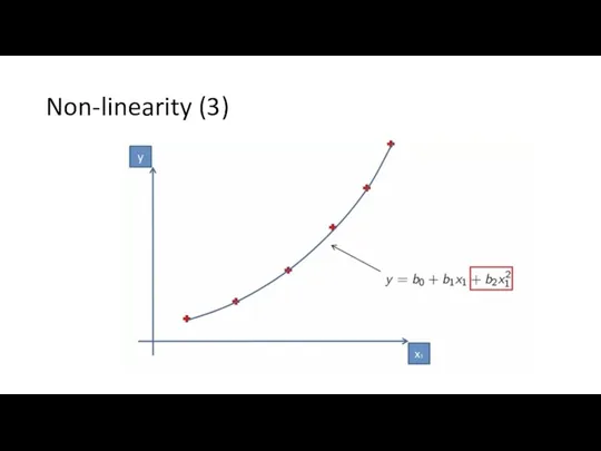
Non-linearity (3)
Non-linearity (3)
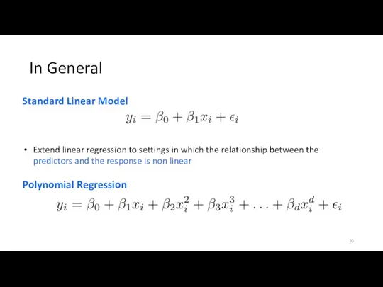
In General
Standard Linear Model
Extend linear regression to settings in which the
In General
Standard Linear Model
Extend linear regression to settings in which the
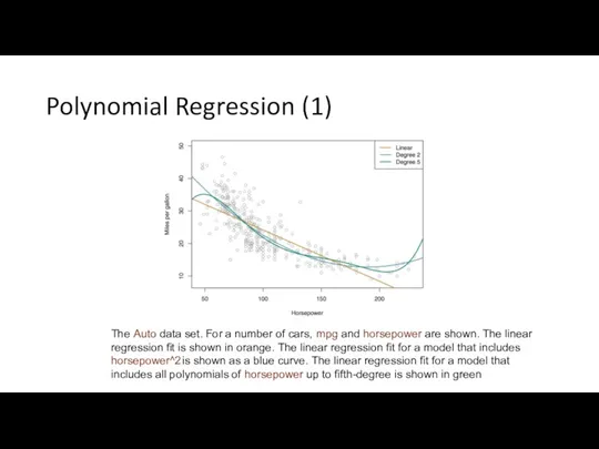
Polynomial Regression (1)
The Auto data set. For a number of cars,
Polynomial Regression (1)
The Auto data set. For a number of cars,
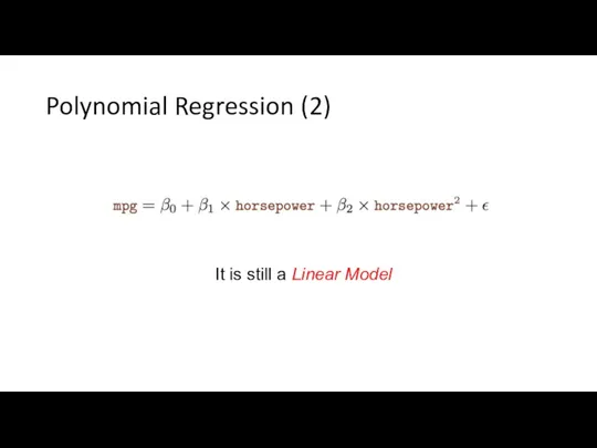
Polynomial Regression (2)
It is still a Linear Model
Polynomial Regression (2)
It is still a Linear Model
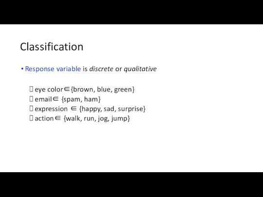
Classification
Response variable is discrete or qualitative
eye color∈{brown, blue, green}
email∈ {spam,
Classification
Response variable is discrete or qualitative
eye color∈{brown, blue, green}
email∈ {spam,
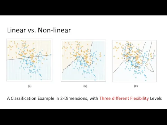
Linear vs. Non-linear
A Classification Example in 2-Dimensions, with Three different Flexibility
Linear vs. Non-linear
A Classification Example in 2-Dimensions, with Three different Flexibility
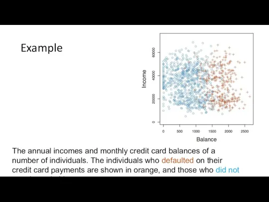
Example
The annual incomes and monthly credit card balances of a number
Example
The annual incomes and monthly credit card balances of a number
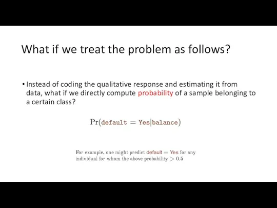
What if we treat the problem as follows?
Instead of coding the
What if we treat the problem as follows?
Instead of coding the
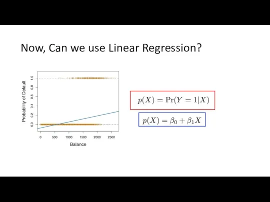
Now, Can we use Linear Regression?
Now, Can we use Linear Regression?
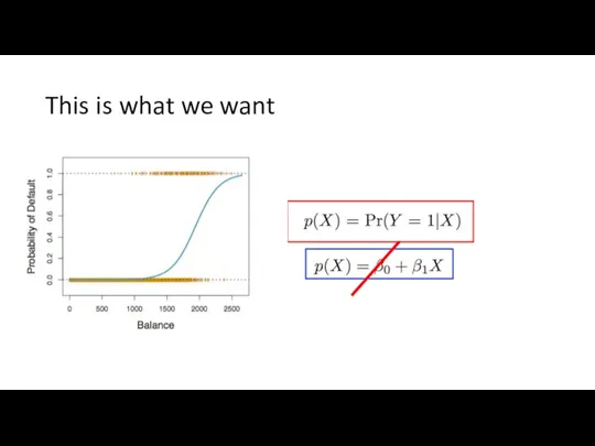
This is what we want
This is what we want
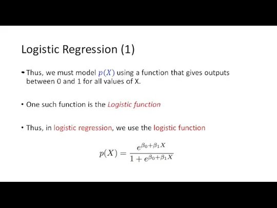
Logistic Regression (1)
Logistic Regression (1)
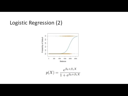
Logistic Regression (2)
Logistic Regression (2)
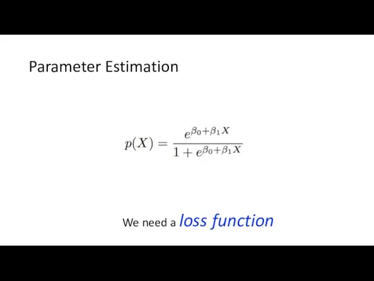
Parameter Estimation
We need a loss function
Parameter Estimation
We need a loss function
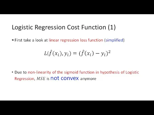
Logistic Regression Cost Function (1)
Logistic Regression Cost Function (1)
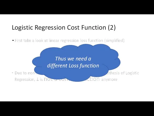
Logistic Regression Cost Function (2)
Thus we need a different Loss function
Logistic Regression Cost Function (2)
Thus we need a different Loss function
Logistic Regression Cost Function (3)
We want to have something that looks
Logistic Regression Cost Function (3)
We want to have something that looks
Logistic Regression Cost Function (4)
Logistic Regression Cost Function (4)
Logistic Regression Cost Function (5)
Logistic Regression Cost Function (5)
Parameter Estimation
Now that we have the cost function, how should we
Parameter Estimation
Now that we have the cost function, how should we
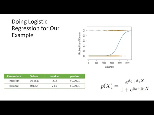
Doing Logistic Regression for Our Example
Doing Logistic Regression for Our Example
Predictions (1)
For example, using the coefficient estimates given in Table 4.1,
Predictions (1)
For example, using the coefficient estimates given in Table 4.1,
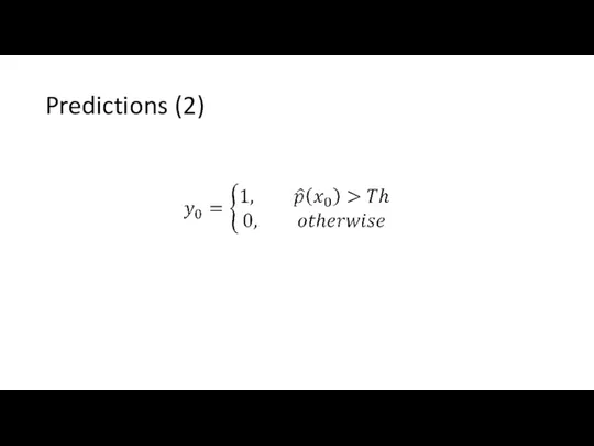
Predictions (2)
Predictions (2)
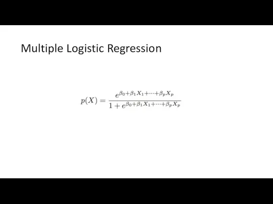
Multiple Logistic Regression
Multiple Logistic Regression
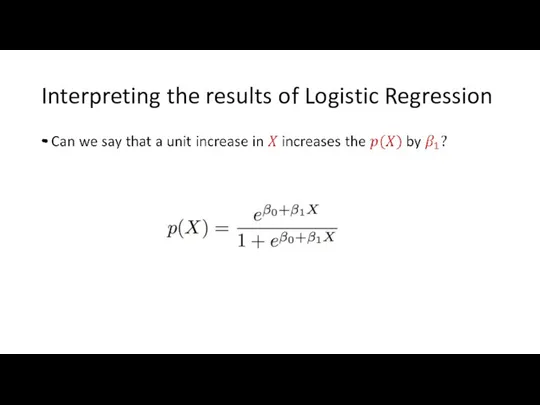
Interpreting the results of Logistic Regression
Interpreting the results of Logistic Regression
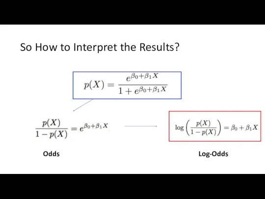
So How to Interpret the Results?
Odds
Log-Odds
So How to Interpret the Results?
Odds
Log-Odds
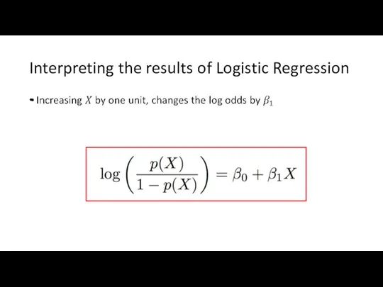
Interpreting the results of Logistic Regression
Interpreting the results of Logistic Regression
Multiclass Classification (1)
One versus All
One versus One
Multiclass Classification (1)
One versus All
One versus One
Multiclass Classification (2)
One versus All
A single multiclass problem is transformed into
Multiclass Classification (2)
One versus All
A single multiclass problem is transformed into
Multiclass Classification (3)
One versus One
A classifier is constructed for each pair
Multiclass Classification (3)
One versus One
A classifier is constructed for each pair
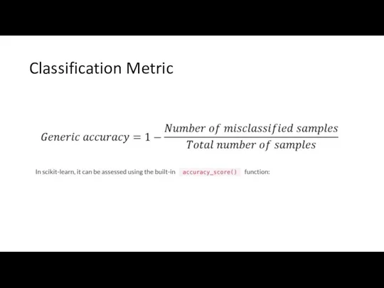
Classification Metric
Classification Metric
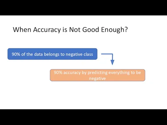
When Accuracy is Not Good Enough?
When Accuracy is Not Good Enough?
Some Simple Requirements for Good Classifier
Better than average classifier
Better than majority
Some Simple Requirements for Good Classifier
Better than average classifier
Better than majority
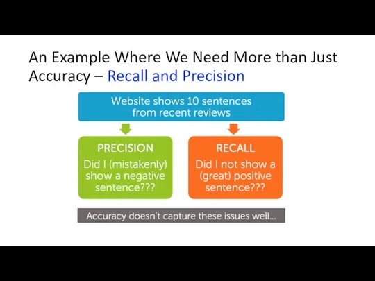
An Example Where We Need More than Just Accuracy – Recall
An Example Where We Need More than Just Accuracy – Recall
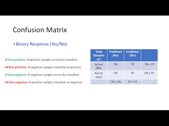
Confusion Matrix
Binary Response (Yes/No)
True positive: A positive sample correctly classified
False positive:
Confusion Matrix
Binary Response (Yes/No)
True positive: A positive sample correctly classified
False positive:
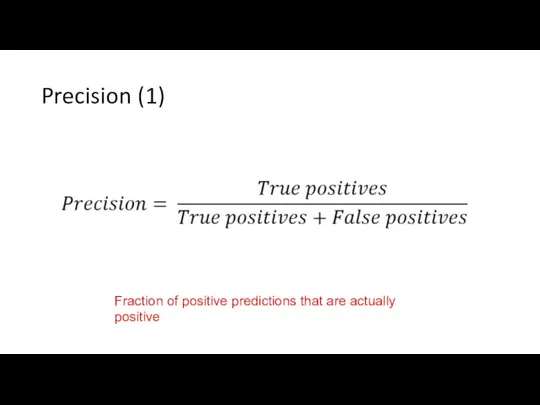
Precision (1)
Fraction of positive predictions that are actually positive
Precision (1)
Fraction of positive predictions that are actually positive
Recall (1)
Fraction of positive data predicted to be positive
Recall (1)
Fraction of positive data predicted to be positive
High Recall Low Precision
Highly Optimistic Model
Predict almost everything as positive
Uses very
High Recall Low Precision
Highly Optimistic Model
Predict almost everything as positive
Uses very
High Precision Low Recall
Highly Pessimistic Model
Predict almost everything as negative
Uses very
High Precision Low Recall
Highly Pessimistic Model
Predict almost everything as negative
Uses very
F-score
Weighted Harmonic Mean b/w Precision and Recall
F-score
Weighted Harmonic Mean b/w Precision and Recall
 Технологии географических информационных систем. Понятие о геоинформатике и ГИС
 Эмоции.Эмоциональные состояния
 Обмен углеводов
 Классный час по теме Символика современных олимпийских игр.
 Нуклеиновые кислоты
 Презентация Сенсорика
 Перспективный план по безопасному поведению детей старшего возраста в детском саду
 Маркетинговые исследования
 Презентация по теме Основания
 Луч и угол
 вокзал
 Классный час Как укрепить иммунитет?
 Дизайн сообществ правки
 Дробные выражения. Устный счет
 Школа вожатых РОО Ритм
 My favorite city is Cherepovets
 Музыкальная образовательная деятельность Путешествие в мир музыкальных инструментов с ИКТ
 Должностные статусы, ученые степени и звания Президента Н. А. Назарбаева
 презентация опыта
 Классификация фенольных соединений
 Шигеллалар
 Сказка об этикете 2.
 Гигиенические требования к планировке, благоустройству и содержанию жилья
 Кольорова металургія
 Синхронные генераторы
 загадки на 23 февраля
 Балық жартылай фабрикаттарын және балық өнімдерін сақтау және сапасын анықтау
 Проектирование на базе программно-технического комплекса АРС