- Operating and Financial Leverage

Содержание
- 2. After studying Chapter 16, you should be able to: Define operating and financial leverage and identify
- 3. Operating and Financial Leverage Operating Leverage Financial Leverage Total Leverage Cash-Flow Ability to Service Debt Other
- 4. Operating Leverage One potential “effect” caused by the presence of operating leverage is that a change
- 5. Impact of Operating Leverage on Profits Firm F Firm V Firm 2F Sales $10 $11 $19.5
- 6. Impact of Operating Leverage on Profits Now, subject each firm to a 50% increase in sales
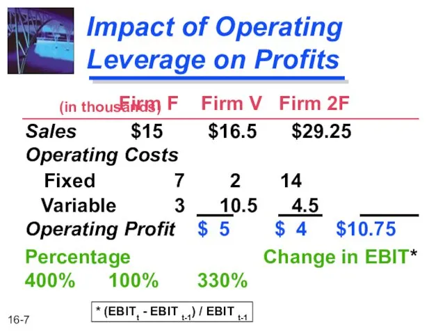
- 7. Impact of Operating Leverage on Profits Firm F Firm V Firm 2F Sales $15 $16.5 $29.25
- 8. Impact of Operating Leverage on Profits Firm F is the most “sensitive” firm -- for it,
- 9. Break-Even Analysis When studying operating leverage, “profits” refers to operating profits before taxes (i.e., EBIT) and
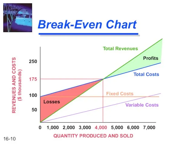
- 10. Break-Even Chart QUANTITY PRODUCED AND SOLD 0 1,000 2,000 3,000 4,000 5,000 6,000 7,000 Total Revenues
- 11. Break-Even (Quantity) Point How to find the quantity break-even point: EBIT = P(Q) - V(Q) -
- 12. Break-Even (Quantity) Point Breakeven occurs when EBIT = 0 Q (P - V) - FC =
- 13. Break-Even (Sales) Point How to find the sales break-even point: SBE = FC + (VCBE) SBE
- 14. Break-Even Point Example Basket Wonders (BW) wants to determine both the quantity and sales break-even points
- 15. Break-Even Point (s) Breakeven occurs when: QBE = FC / (P - V) QBE = $100,000
- 16. Break-Even Chart QUANTITY PRODUCED AND SOLD 0 1,000 2,000 3,000 4,000 5,000 6,000 7,000 Total Revenues
- 17. Degree of Operating Leverage (DOL) DOL at Q units of output (or sales) Degree of Operating
- 18. Computing the DOL DOLQ units Calculating the DOL for a single product or a single-product firm.
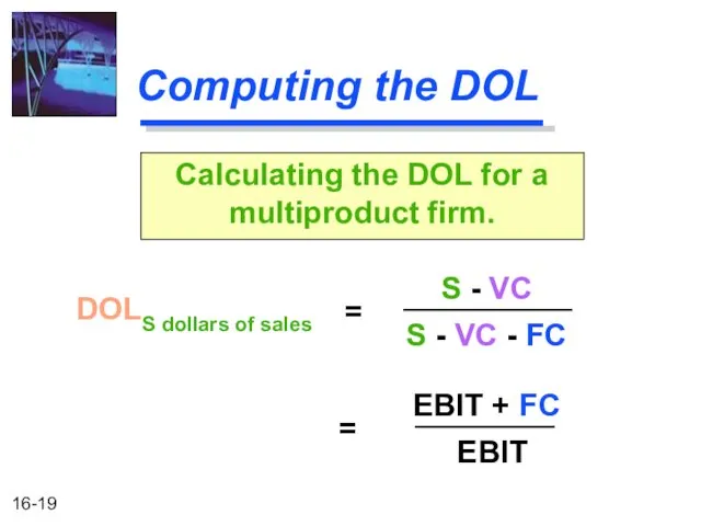
- 19. Computing the DOL DOLS dollars of sales Calculating the DOL for a multiproduct firm. = S
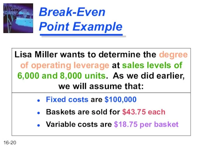
- 20. Break-Even Point Example Lisa Miller wants to determine the degree of operating leverage at sales levels
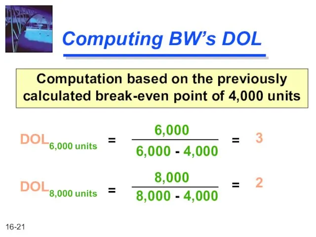
- 21. Computing BW’s DOL DOL6,000 units Computation based on the previously calculated break-even point of 4,000 units
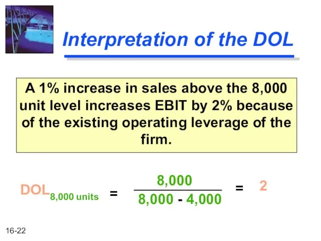
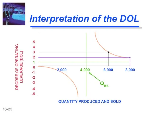
- 22. Interpretation of the DOL A 1% increase in sales above the 8,000 unit level increases EBIT
- 23. Interpretation of the DOL 2,000 4,000 6,000 8,000 1 2 3 4 5 QUANTITY PRODUCED AND
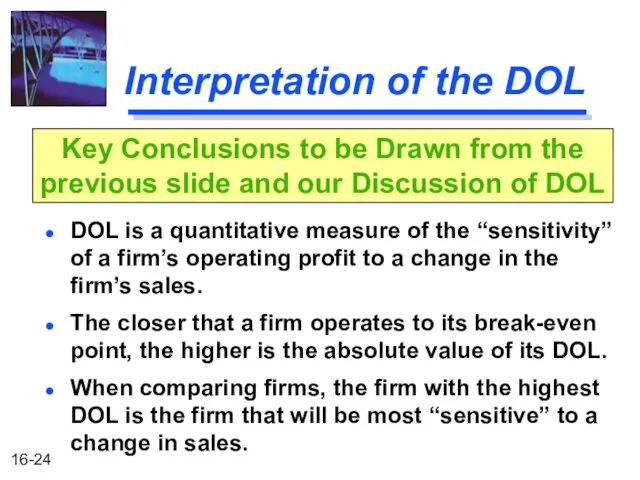
- 24. Interpretation of the DOL DOL is a quantitative measure of the “sensitivity” of a firm’s operating
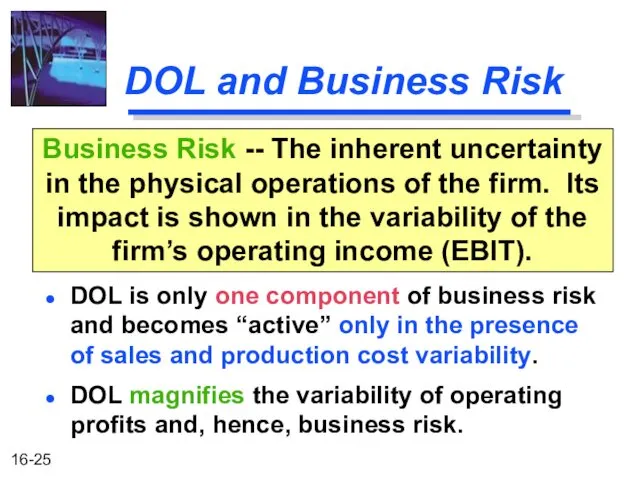
- 25. DOL and Business Risk DOL is only one component of business risk and becomes “active” only
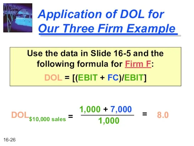
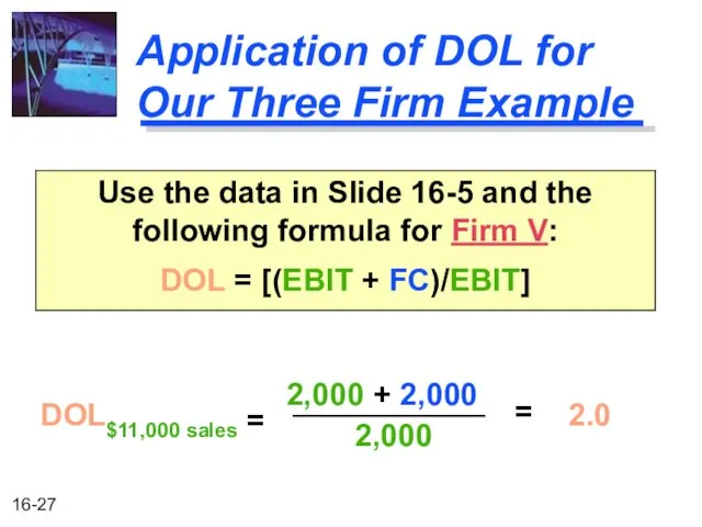
- 26. Application of DOL for Our Three Firm Example Use the data in Slide 16-5 and the
- 27. Application of DOL for Our Three Firm Example Use the data in Slide 16-5 and the
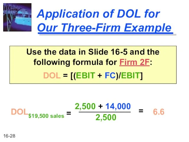
- 28. Application of DOL for Our Three-Firm Example Use the data in Slide 16-5 and the following
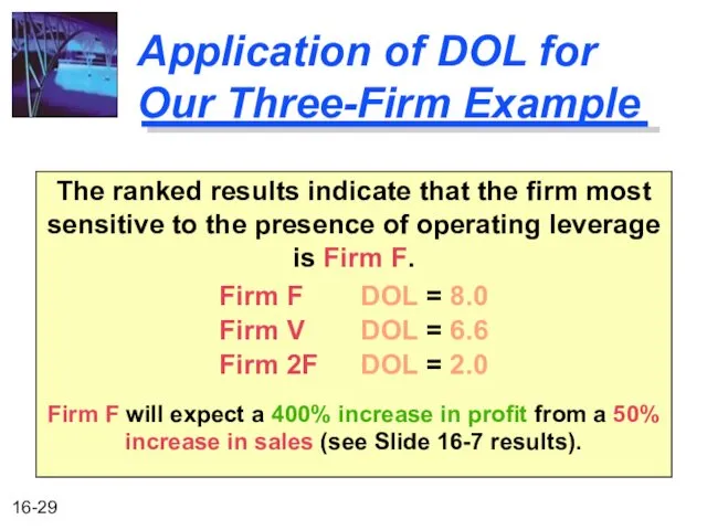
- 29. Application of DOL for Our Three-Firm Example The ranked results indicate that the firm most sensitive
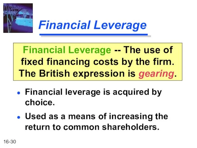
- 30. Financial Leverage Financial leverage is acquired by choice. Used as a means of increasing the return
- 31. EBIT-EPS Break-Even, or Indifference, Analysis Calculate EPS for a given level of EBIT at a given
- 32. EBIT-EPS Chart Current common equity shares = 50,000 $1 million in new financing of either: All
- 33. EBIT-EPS Calculation with New Equity Financing EBIT $500,000 $150,000* Interest 0 0 EBT $500,000 $150,000 Taxes
- 34. EBIT-EPS Chart 0 100 200 300 400 500 600 700 EBIT ($ thousands) Earnings per Share
- 35. EBIT-EPS Calculation with New Debt Financing EBIT $500,000 $150,000* Interest 100,000 100,000 EBT $400,000 $ 50,000
- 36. EBIT-EPS Chart 0 100 200 300 400 500 600 700 EBIT ($ thousands) Earnings per Share
- 37. EBIT-EPS Calculation with New Preferred Financing EBIT $500,000 $150,000* Interest 0 0 EBT $500,000 $150,000 Taxes
- 38. 0 100 200 300 400 500 600 700 EBIT-EPS Chart EBIT ($ thousands) Earnings per Share
- 39. What About Risk? 0 100 200 300 400 500 600 700 EBIT ($ thousands) Earnings per
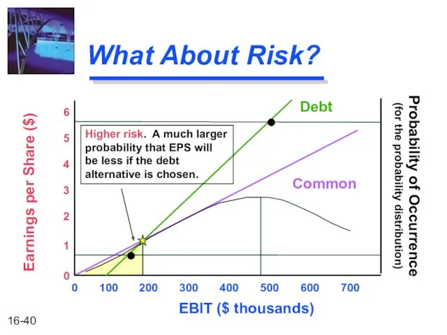
- 40. What About Risk? 0 100 200 300 400 500 600 700 EBIT ($ thousands) Earnings per
- 41. Degree of Financial Leverage (DFL) DFL at EBIT of X dollars Degree of Financial Leverage --
- 42. Computing the DFL DFL EBIT of $X Calculating the DFL = EBIT EBIT - I -
- 43. What is the DFL for Each of the Financing Choices? DFL $500,000 Calculating the DFL for
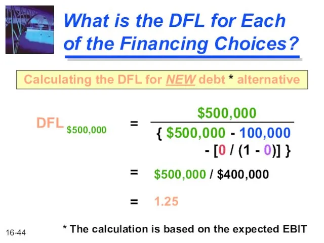
- 44. What is the DFL for Each of the Financing Choices? DFL $500,000 Calculating the DFL for
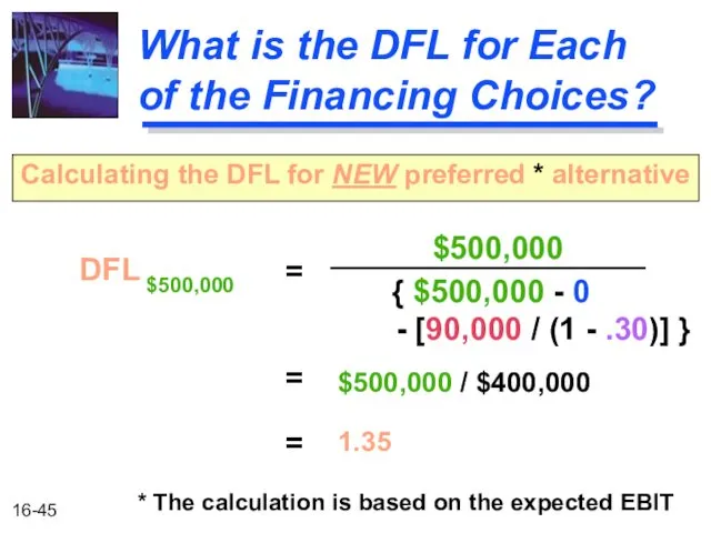
- 45. What is the DFL for Each of the Financing Choices? DFL $500,000 Calculating the DFL for
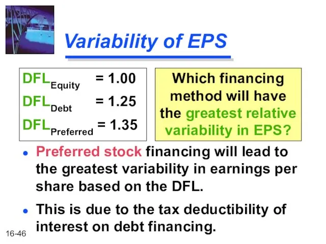
- 46. Variability of EPS Preferred stock financing will lead to the greatest variability in earnings per share
- 47. Financial Risk Debt increases the probability of cash insolvency over an all-equity-financed firm. For example, our
- 48. Total Firm Risk CVEPS is a measure of relative total firm risk CVEBIT is a measure
- 49. Degree of Total Leverage (DTL) DTL at Q units (or S dollars) of output (or sales)
- 50. Computing the DTL DTL S dollars of sales DTL Q units (or S dollars) = (
- 51. DTL Example Lisa Miller wants to determine the Degree of Total Leverage at EBIT=$500,000. As we
- 52. Computing the DTL for All-Equity Financing DTL S dollars of sales = $500,000 + $100,000 $500,000
- 53. Computing the DTL for Debt Financing DTL S dollars of sales = $500,000 + $100,000 {
- 54. Risk versus Return Compare the expected EPS to the DTL for the common stock equity financing
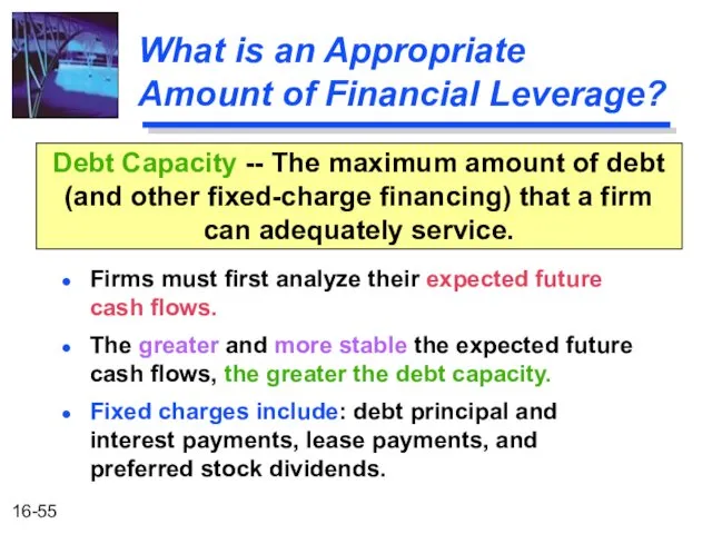
- 55. What is an Appropriate Amount of Financial Leverage? Firms must first analyze their expected future cash
- 56. Coverage Ratios Interest Coverage EBIT Interest expenses Indicates a firm’s ability to cover interest charges. Income
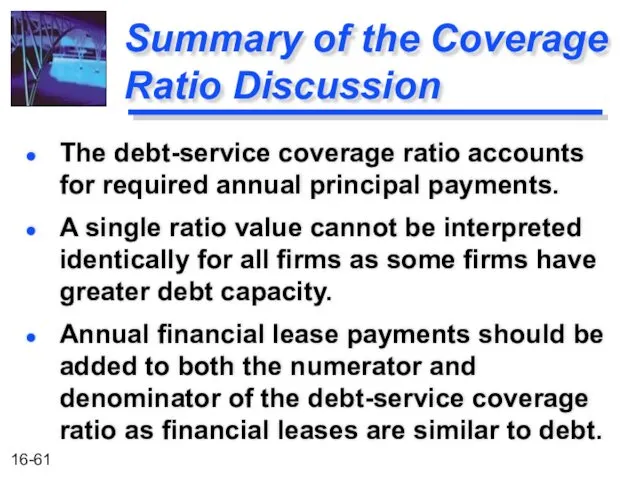
- 57. Coverage Ratios Debt-service Coverage EBIT { Interest expenses + [Principal payments / (1-t) ] } Indicates
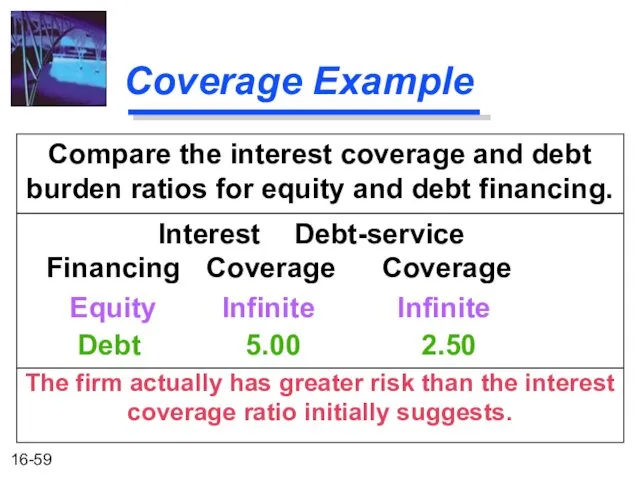
- 58. Coverage Example Make an examination of the coverage ratios for Basket Wonders when EBIT=$500,000. Compare the
- 59. Coverage Example Compare the interest coverage and debt burden ratios for equity and debt financing. Interest
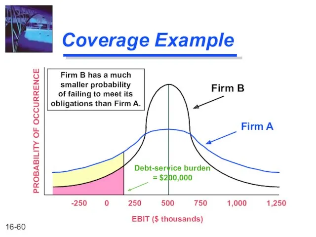
- 60. Coverage Example -250 0 250 500 750 1,000 1,250 EBIT ($ thousands) Firm B has a
- 61. Summary of the Coverage Ratio Discussion A single ratio value cannot be interpreted identically for all
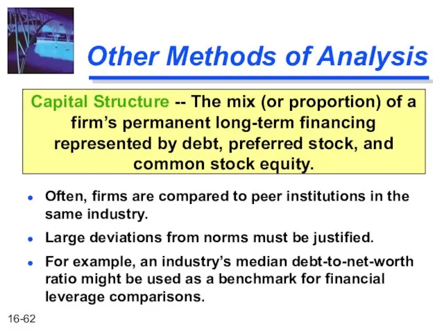
- 62. Other Methods of Analysis Often, firms are compared to peer institutions in the same industry. Large
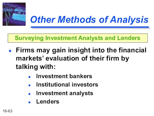
- 63. Other Methods of Analysis Firms may gain insight into the financial markets’ evaluation of their firm
- 65. Скачать презентацию
After studying Chapter 16, you should be able to:
Define operating and
After studying Chapter 16, you should be able to:
Define operating and
Operating and Financial Leverage
Operating Leverage
Financial Leverage
Total Leverage
Cash-Flow Ability to Service Debt
Other
Operating and Financial Leverage
Operating Leverage
Financial Leverage
Total Leverage
Cash-Flow Ability to Service Debt
Other
Operating Leverage
One potential “effect” caused by the presence of operating leverage
Operating Leverage
One potential “effect” caused by the presence of operating leverage

Impact of Operating Leverage on Profits
Firm F Firm V Firm
Impact of Operating Leverage on Profits
Firm F Firm V Firm
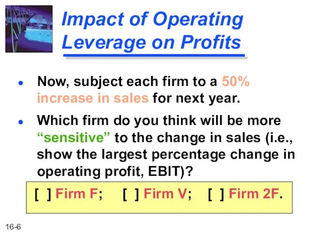
Impact of Operating Leverage on Profits
Now, subject each firm to a
Impact of Operating Leverage on Profits
Now, subject each firm to a
Impact of Operating Leverage on Profits
Firm F Firm V Firm
Impact of Operating Leverage on Profits
Firm F Firm V Firm
Impact of Operating Leverage on Profits
Firm F is the most “sensitive”
Impact of Operating Leverage on Profits
Firm F is the most “sensitive”
Break-Even Analysis
When studying operating leverage, “profits” refers to operating profits before
Break-Even Analysis
When studying operating leverage, “profits” refers to operating profits before
Break-Even Chart
QUANTITY PRODUCED AND SOLD
0 1,000 2,000 3,000 4,000 5,000 6,000
Break-Even Chart
QUANTITY PRODUCED AND SOLD
0 1,000 2,000 3,000 4,000 5,000 6,000
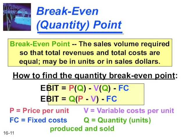
Break-Even (Quantity) Point
How to find the quantity break-even point:
EBIT =
Break-Even (Quantity) Point
How to find the quantity break-even point:
EBIT =
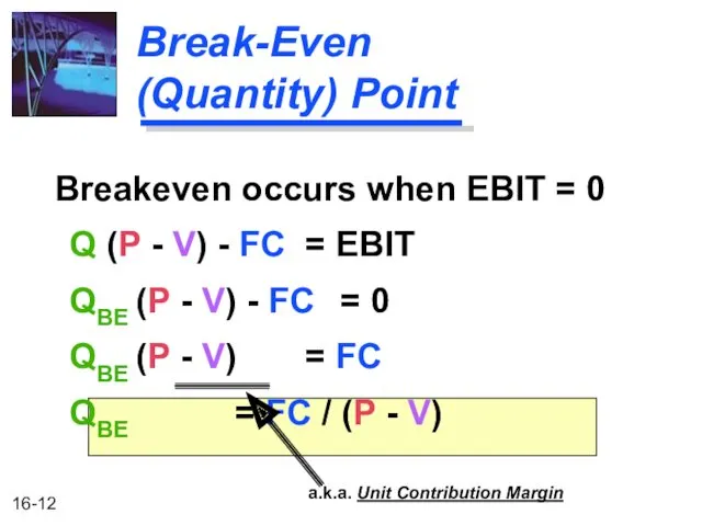
Break-Even (Quantity) Point
Breakeven occurs when EBIT = 0
Q (P -
Break-Even (Quantity) Point
Breakeven occurs when EBIT = 0
Q (P -
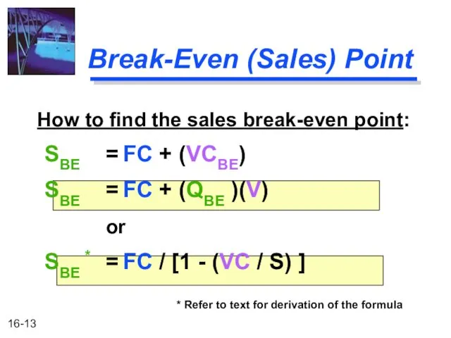
Break-Even (Sales) Point
How to find the sales break-even point:
SBE =
Break-Even (Sales) Point
How to find the sales break-even point:
SBE =
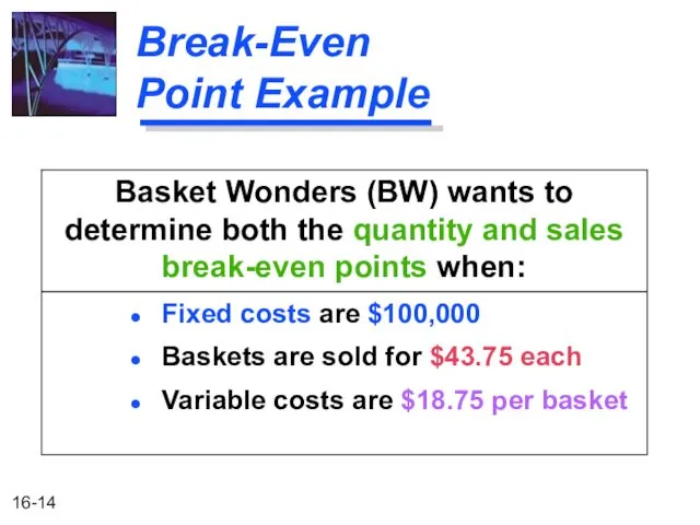
Break-Even Point Example
Basket Wonders (BW) wants to determine both the quantity
Break-Even Point Example
Basket Wonders (BW) wants to determine both the quantity
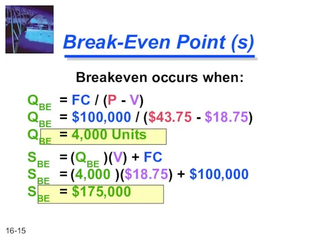
Break-Even Point (s)
Breakeven occurs when:
QBE = FC / (P - V)
Break-Even Point (s)
Breakeven occurs when:
QBE = FC / (P - V)
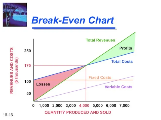
Break-Even Chart
QUANTITY PRODUCED AND SOLD
0 1,000 2,000 3,000 4,000 5,000 6,000
Break-Even Chart
QUANTITY PRODUCED AND SOLD
0 1,000 2,000 3,000 4,000 5,000 6,000
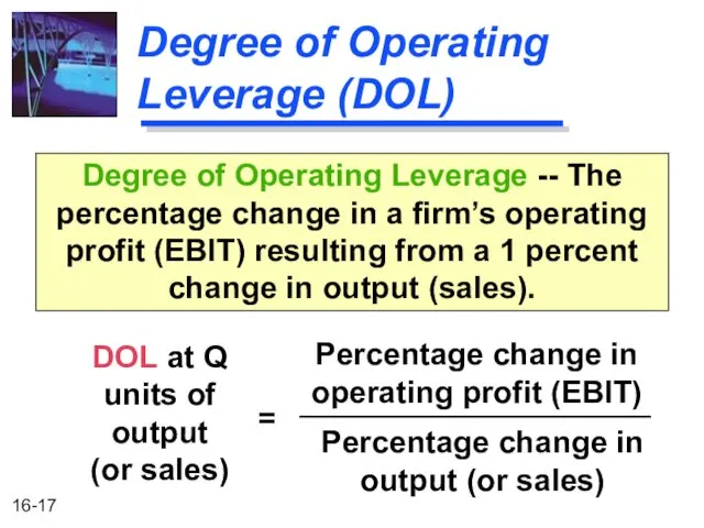
Degree of Operating Leverage (DOL)
DOL at Q units of output
(or
Degree of Operating Leverage (DOL)
DOL at Q units of output
(or
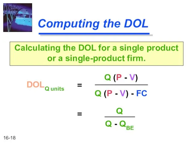
Computing the DOL
DOLQ units
Calculating the DOL for a single product or
Computing the DOL
DOLQ units
Calculating the DOL for a single product or
Computing the DOL
DOLS dollars of sales
Calculating the DOL for a multiproduct
Computing the DOL
DOLS dollars of sales
Calculating the DOL for a multiproduct
Break-Even Point Example
Lisa Miller wants to determine the degree of operating
Break-Even Point Example
Lisa Miller wants to determine the degree of operating
Computing BW’s DOL
DOL6,000 units
Computation based on the previously calculated break-even point
Computing BW’s DOL
DOL6,000 units
Computation based on the previously calculated break-even point
Interpretation of the DOL
A 1% increase in sales above the 8,000
Interpretation of the DOL
A 1% increase in sales above the 8,000
Interpretation of the DOL
2,000 4,000 6,000 8,000
1
2
3
4
5
QUANTITY PRODUCED AND SOLD
0
-1
-2
-3
-4
-5
DEGREE OF
Interpretation of the DOL
2,000 4,000 6,000 8,000
1
2
3
4
5
QUANTITY PRODUCED AND SOLD
0
-1
-2
-3
-4
-5
DEGREE OF
Interpretation of the DOL
DOL is a quantitative measure of the “sensitivity”
Interpretation of the DOL
DOL is a quantitative measure of the “sensitivity”
DOL and Business Risk
DOL is only one component of business risk
DOL and Business Risk
DOL is only one component of business risk
Application of DOL for Our Three Firm Example
Use the data in
Application of DOL for Our Three Firm Example
Use the data in
Application of DOL for Our Three Firm Example
Use the data in
Application of DOL for Our Three Firm Example
Use the data in
Application of DOL for Our Three-Firm Example
Use the data in Slide
Application of DOL for Our Three-Firm Example
Use the data in Slide
Application of DOL for Our Three-Firm Example
The ranked results indicate that
Application of DOL for Our Three-Firm Example
The ranked results indicate that
Financial Leverage
Financial leverage is acquired by choice.
Used as a means of
Financial Leverage
Financial leverage is acquired by choice.
Used as a means of
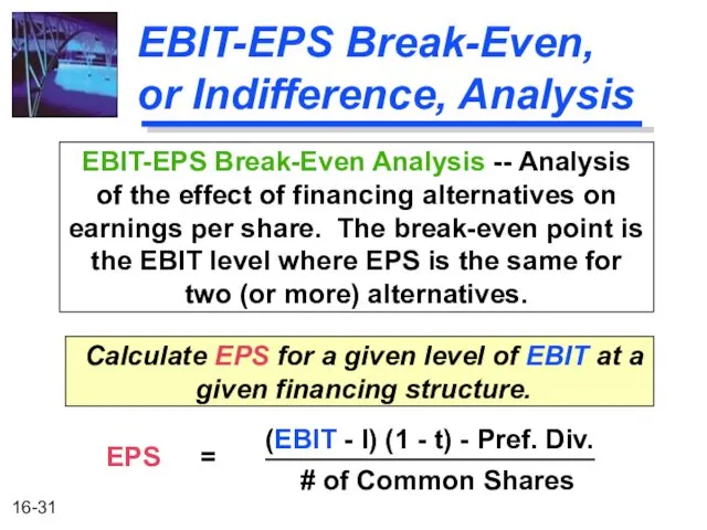
EBIT-EPS Break-Even, or Indifference, Analysis
Calculate EPS for a given level of
EBIT-EPS Break-Even, or Indifference, Analysis
Calculate EPS for a given level of
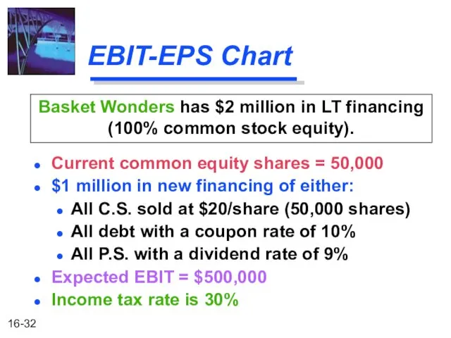
EBIT-EPS Chart
Current common equity shares = 50,000
$1 million in new financing
EBIT-EPS Chart
Current common equity shares = 50,000
$1 million in new financing
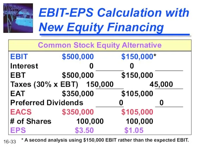
EBIT-EPS Calculation with New Equity Financing
EBIT $500,000 $150,000*
Interest 0 0
EBT $500,000
EBIT-EPS Calculation with New Equity Financing
EBIT $500,000 $150,000*
Interest 0 0
EBT $500,000
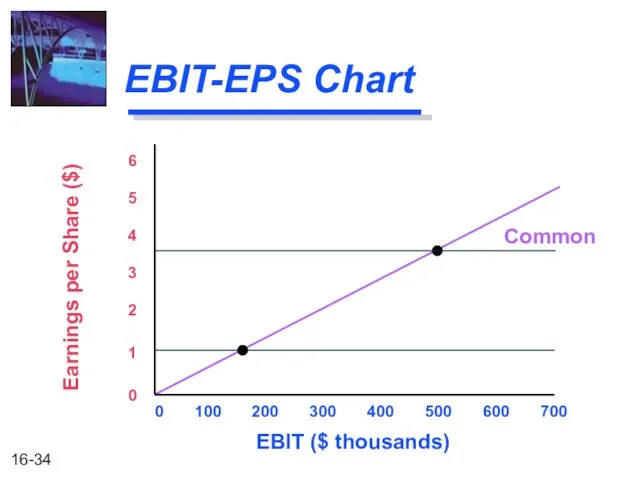
EBIT-EPS Chart
0 100 200 300 400 500 600 700
EBIT ($ thousands)
Earnings
EBIT-EPS Chart
0 100 200 300 400 500 600 700
EBIT ($ thousands)
Earnings
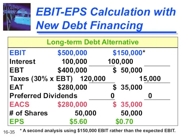
EBIT-EPS Calculation with New Debt Financing
EBIT $500,000 $150,000*
Interest 100,000 100,000
EBT $400,000
EBIT-EPS Calculation with New Debt Financing
EBIT $500,000 $150,000*
Interest 100,000 100,000
EBT $400,000
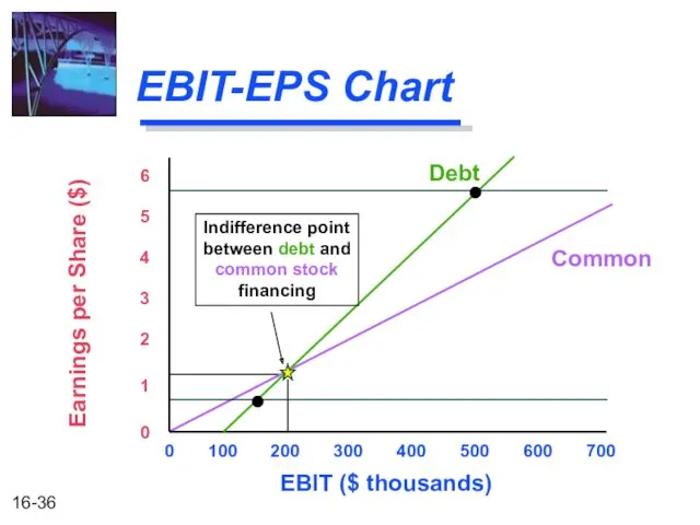
EBIT-EPS Chart
0 100 200 300 400 500 600 700
EBIT ($ thousands)
Earnings
EBIT-EPS Chart
0 100 200 300 400 500 600 700
EBIT ($ thousands)
Earnings
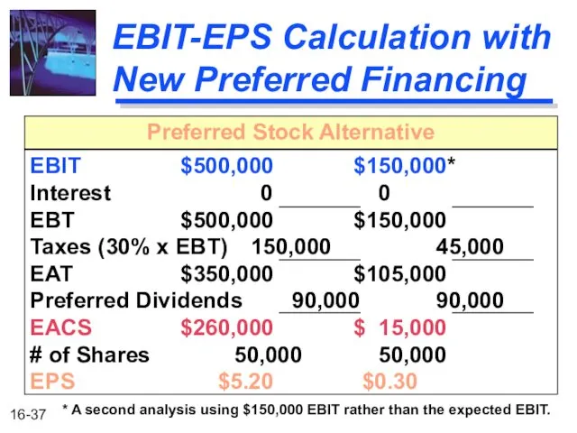
EBIT-EPS Calculation with New Preferred Financing
EBIT $500,000 $150,000*
Interest 0 0
EBT $500,000
EBIT-EPS Calculation with New Preferred Financing
EBIT $500,000 $150,000*
Interest 0 0
EBT $500,000
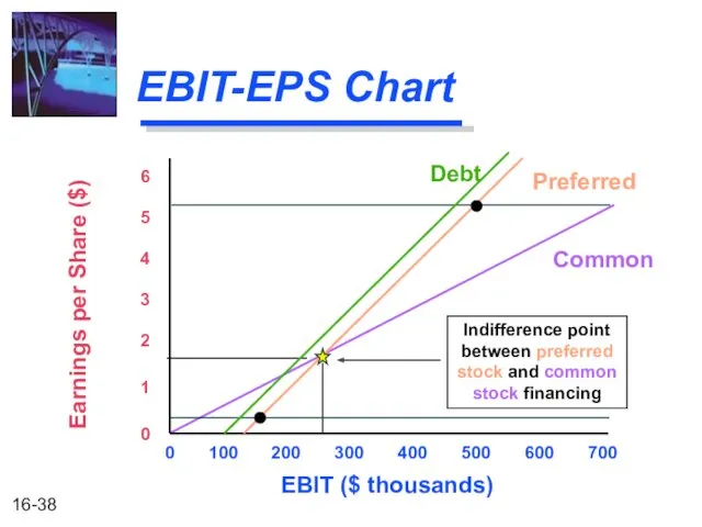
0 100 200 300 400 500 600 700
EBIT-EPS Chart
EBIT ($ thousands)
Earnings
0 100 200 300 400 500 600 700
EBIT-EPS Chart
EBIT ($ thousands)
Earnings
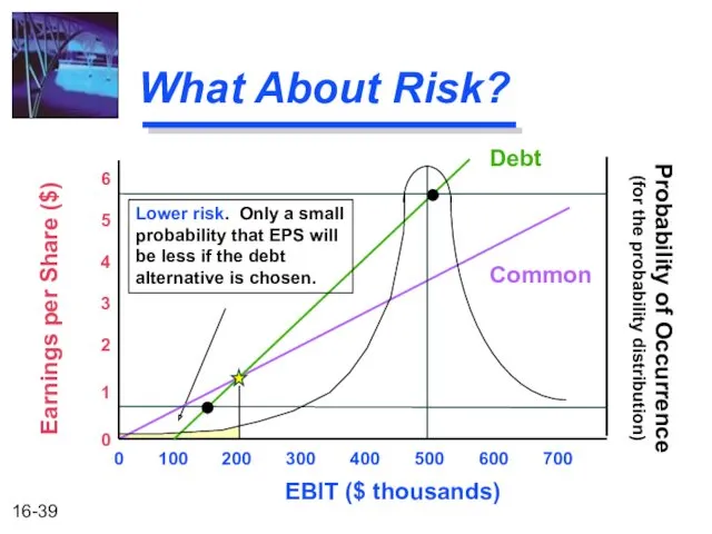
What About Risk?
0 100 200 300 400 500 600 700
EBIT ($
What About Risk?
0 100 200 300 400 500 600 700
EBIT ($
What About Risk?
0 100 200 300 400 500 600 700
EBIT ($
What About Risk?
0 100 200 300 400 500 600 700
EBIT ($
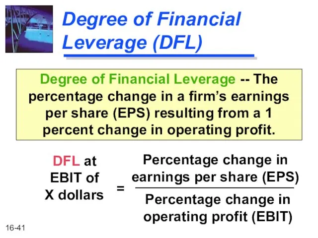
Degree of Financial Leverage (DFL)
DFL at EBIT of X dollars
Degree of
Degree of Financial Leverage (DFL)
DFL at EBIT of X dollars
Degree of
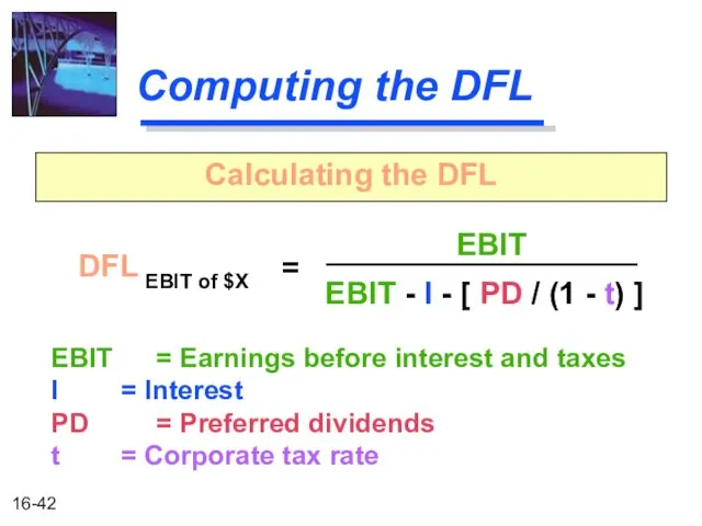
Computing the DFL
DFL EBIT of $X
Calculating the DFL
=
EBIT
EBIT - I -
Computing the DFL
DFL EBIT of $X
Calculating the DFL
=
EBIT
EBIT - I -
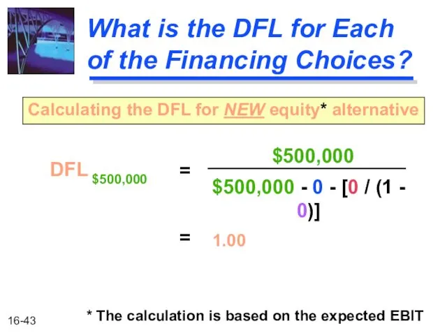
What is the DFL for Each of the Financing Choices?
DFL $500,000
Calculating
What is the DFL for Each of the Financing Choices?
DFL $500,000
Calculating
What is the DFL for Each of the Financing Choices?
DFL $500,000
Calculating
What is the DFL for Each of the Financing Choices?
DFL $500,000
Calculating
What is the DFL for Each of the Financing Choices?
DFL $500,000
Calculating
What is the DFL for Each of the Financing Choices?
DFL $500,000
Calculating
Variability of EPS
Preferred stock financing will lead to the greatest variability
Variability of EPS
Preferred stock financing will lead to the greatest variability
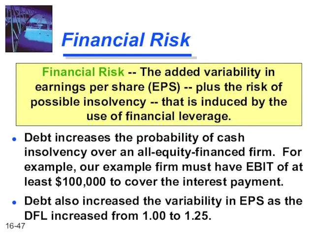
Financial Risk
Debt increases the probability of cash insolvency over an all-equity-financed
Financial Risk
Debt increases the probability of cash insolvency over an all-equity-financed
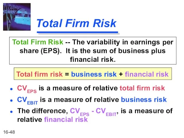
Total Firm Risk
CVEPS is a measure of relative total firm risk
CVEBIT
Total Firm Risk
CVEPS is a measure of relative total firm risk
CVEBIT
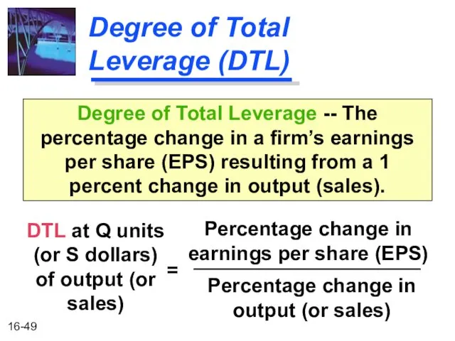
Degree of Total Leverage (DTL)
DTL at Q units (or S dollars)
Degree of Total Leverage (DTL)
DTL at Q units (or S dollars)
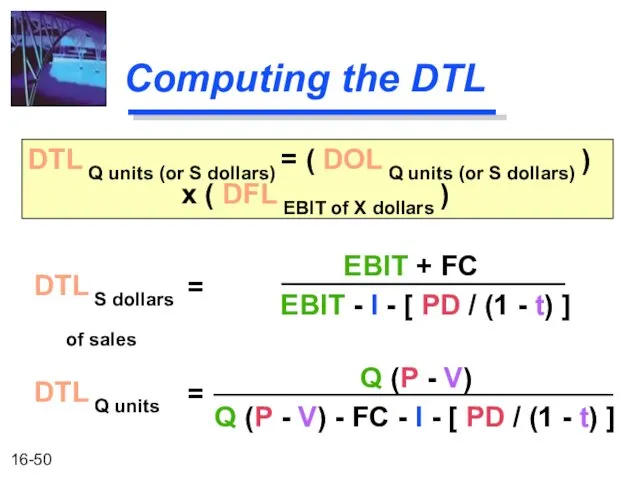
Computing the DTL
DTL S dollars
of sales
DTL Q units (or S dollars)
Computing the DTL
DTL S dollars
of sales
DTL Q units (or S dollars)
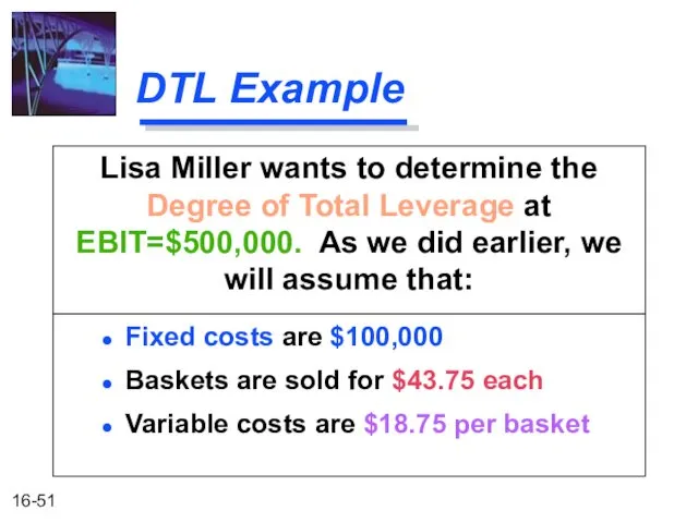
DTL Example
Lisa Miller wants to determine the Degree of Total Leverage
DTL Example
Lisa Miller wants to determine the Degree of Total Leverage
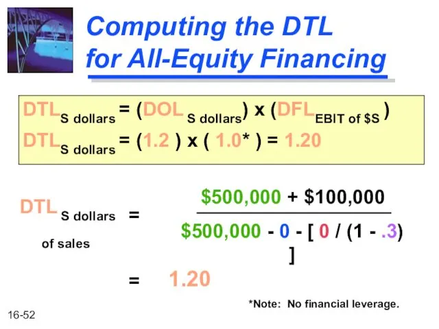
Computing the DTL
for All-Equity Financing
DTL S dollars
of sales
=
$500,000 + $100,000
$500,000
Computing the DTL
for All-Equity Financing
DTL S dollars
of sales
=
$500,000 + $100,000
$500,000
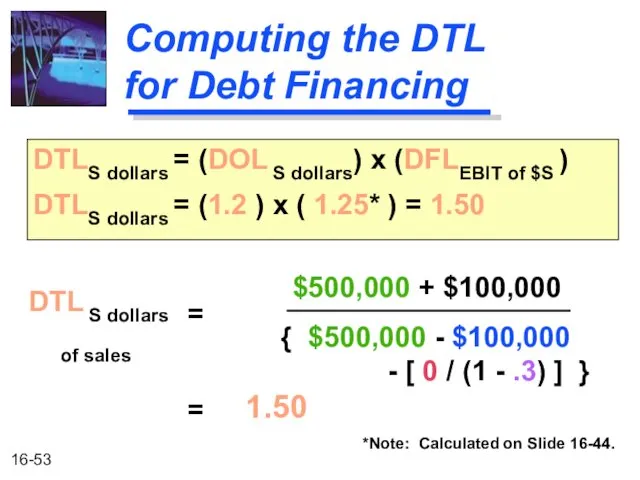
Computing the DTL
for Debt Financing
DTL S dollars
of sales
=
$500,000 + $100,000
{
Computing the DTL
for Debt Financing
DTL S dollars
of sales
=
$500,000 + $100,000
{
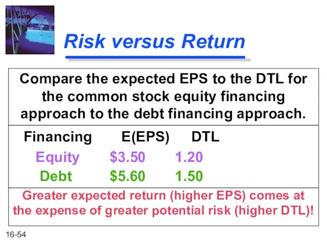
Risk versus Return
Compare the expected EPS to the DTL for the
Risk versus Return
Compare the expected EPS to the DTL for the
What is an Appropriate
Amount of Financial Leverage?
Firms must first analyze
What is an Appropriate
Amount of Financial Leverage?
Firms must first analyze
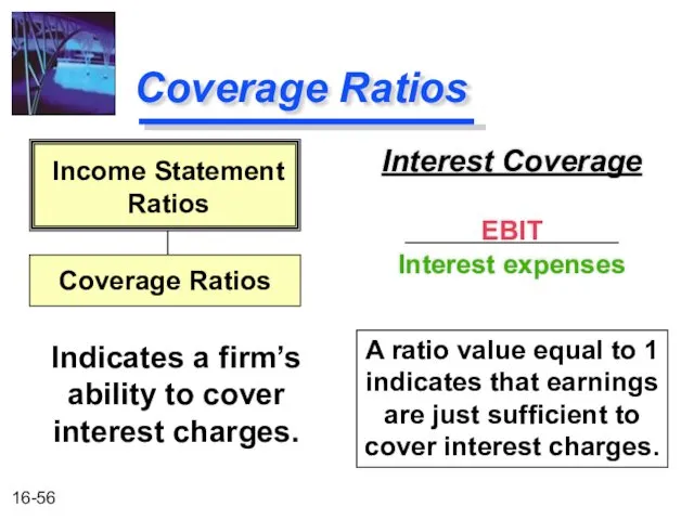
Coverage Ratios
Interest Coverage
EBIT
Interest expenses
Indicates a firm’s ability to cover interest charges.
Income
Coverage Ratios
Interest Coverage
EBIT
Interest expenses
Indicates a firm’s ability to cover interest charges.
Income
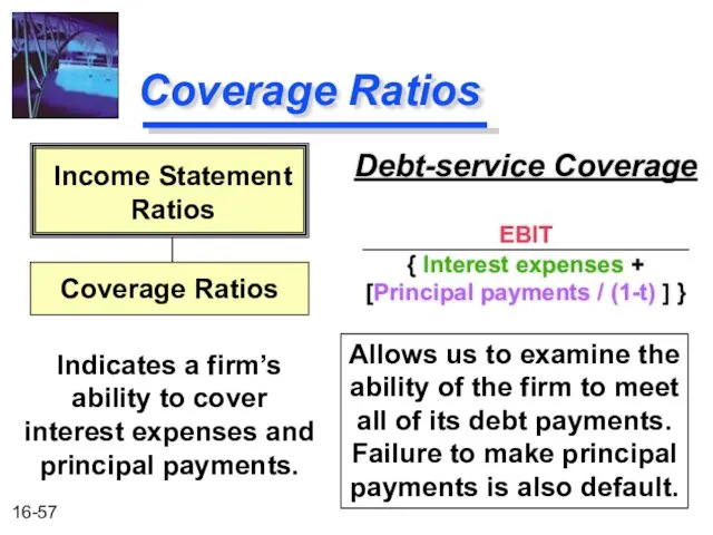
Coverage Ratios
Debt-service Coverage
EBIT
{ Interest expenses + [Principal payments / (1-t) ]
Coverage Ratios
Debt-service Coverage
EBIT
{ Interest expenses + [Principal payments / (1-t) ]
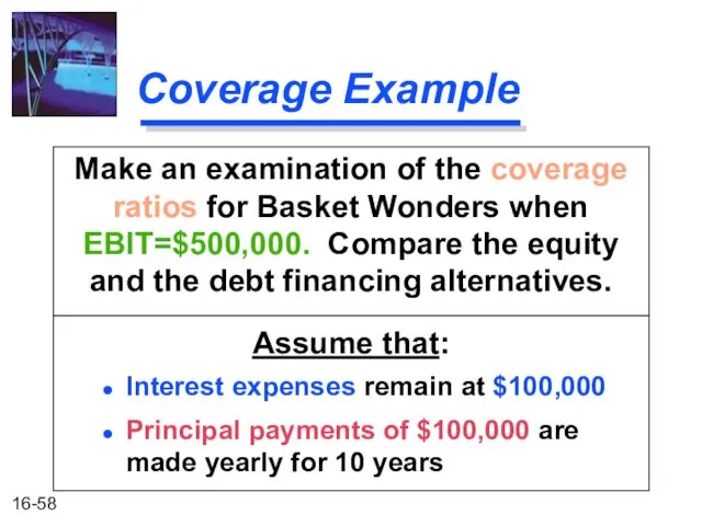
Coverage Example
Make an examination of the coverage ratios for Basket Wonders
Coverage Example
Make an examination of the coverage ratios for Basket Wonders
Coverage Example
Compare the interest coverage and debt burden ratios for equity
Coverage Example
Compare the interest coverage and debt burden ratios for equity
Coverage Example
-250 0 250 500 750 1,000 1,250
EBIT ($ thousands)
Firm B
Coverage Example
-250 0 250 500 750 1,000 1,250
EBIT ($ thousands)
Firm B
Summary of the Coverage Ratio Discussion
A single ratio value cannot be
Summary of the Coverage Ratio Discussion
A single ratio value cannot be
Other Methods of Analysis
Often, firms are compared to peer institutions in
Other Methods of Analysis
Often, firms are compared to peer institutions in
Other Methods of Analysis
Firms may gain insight into the financial markets’
Other Methods of Analysis
Firms may gain insight into the financial markets’
 Презентация о моей работе
 Оценка качества зданий. Показатели качества зданий. Обследование зданий
 Вокальная музыка. (5 класс)
 Заповедники и славянофилы
 Основные понятия и определения делопроизводства
 Тайна имени
 Пивоварня Anchor
 Математическое моделирование и численные методы в инженерных задачах
 Основы генетики
 Контроль, как функция менеджмента. (Тема 12)
 Омонимы разработка урока по татарскому языку.
 Сдай макулатуру спаси дерево Сережкина (1)
 Прощай Букварь! Сау бул Әлифба!
 17424-ulitsy-goroda-tambova-vosstanovlen.pptx
 Континент Антарктида
 Мастер - класс для родителей Народная кукла - как источник развития ребёнка
 Презентация по татарскому языку 2 класс. Тема Шәхси гигиена.
 Витамины - общая характеристика.
 Ислам діні.Суннит
 Презентация Путешествие Лунтика по планете Земля
 Ферменты (10 класс)
 Технология нанесения антикоррозионных покрытий
 Нефтяная и газовая промышленность
 проектная работа Знакомьтесь - ёжик!
 Мифы о поколении Z
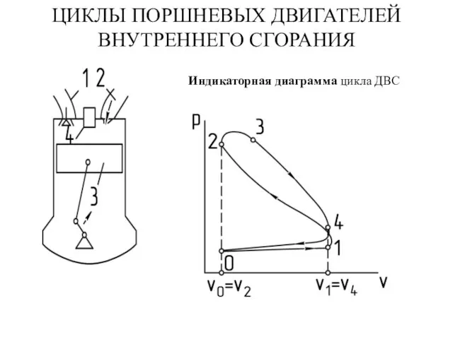 Циклы поршневых двигателей внутреннего сгорания
 Обзор технологий заканчивания скважин для многостадийного ГРП
 Изготовление бахил