- System models

Содержание
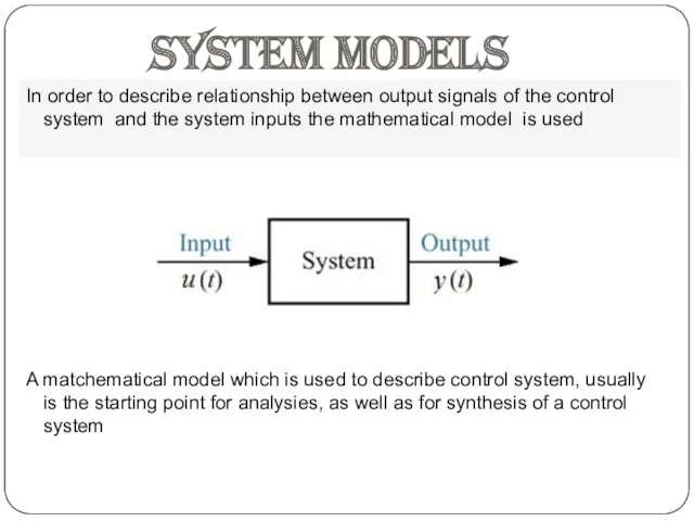
- 2. System models In order to describe relationship between output signals of the control system and the
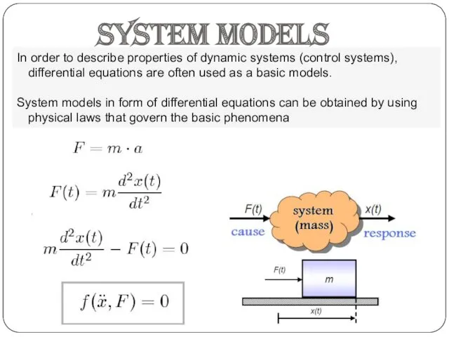
- 3. System models In order to describe properties of dynamic systems (control systems), differential equations are often
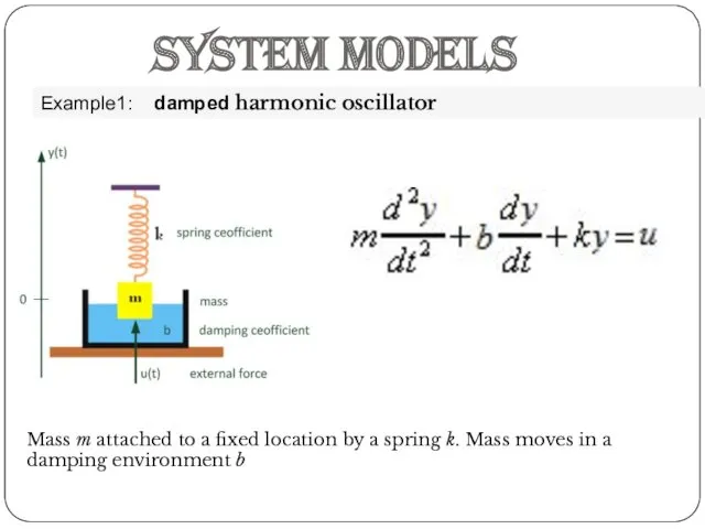
- 4. System models Example1: damped harmonic oscillator Mass m attached to a fixed location by a spring
- 5. Example 2: RC circuit System models From II-nd Kirchhoff's law we can obtain:
- 6. System models Classification of dynamical system models: I. 1. Linear my” + by’ + ky =
- 7. State space models The state space model is an anather way (kind of an ordered way)
- 8. x(t) - state variables, are the smallest possible subset of system variables that can represent the
- 9. State space models If vector functions f and g are linear: Where A is called the
- 10. Example 1 : damped harmonic oscillator Where: is position; is velocity; is acceleration is an applied
- 11. Exercise 2: RC circuit State space models
- 12. The Laplace transform is a linear operation of a function f(t) with a real argument t
- 13. Example 1: Heaviside step function or unit step function Laplace Transform f(t) = 1(t) Exercise 2:
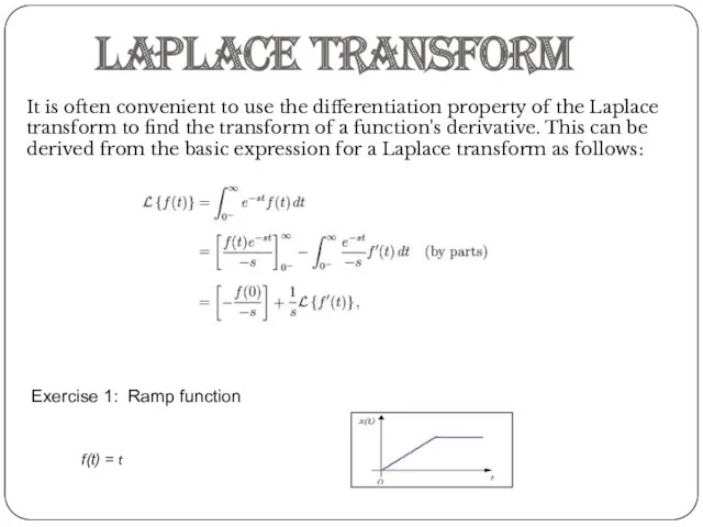
- 14. Laplace Transform It is often convenient to use the differentiation property of the Laplace transform to
- 15. f(t) F(s) Laplace Transform Laplace transforms of typical functions (TABLE OF TRANSFORMS):
- 16. Laplace Transform Laplace transforms of typical functions: f(t) F(s)
- 17. Laplace Transform Laplace transform properties: 1.
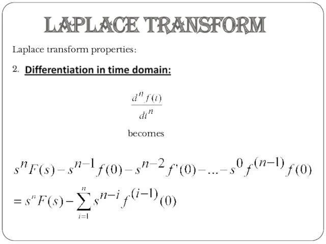
- 18. Laplace Transform Laplace transform properties: 2. becomes
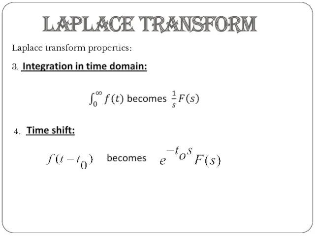
- 19. Laplace Transform Laplace transform properties: 3. 4.
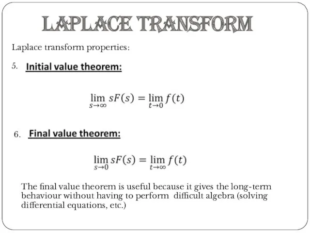
- 20. Laplace Transform Laplace transform properties: 5. 6. The final value theorem is useful because it gives
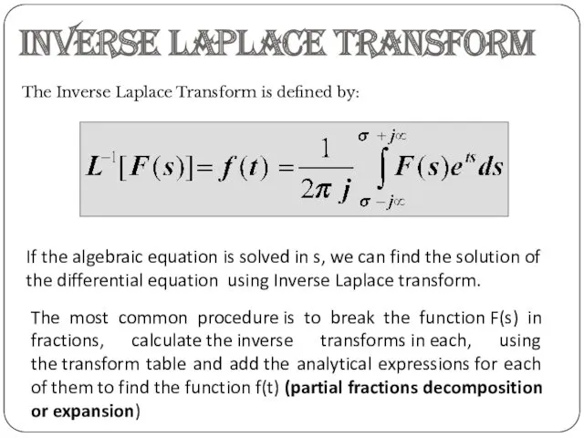
- 21. Inverse Laplace Transform The Inverse Laplace Transform is defined by: If the algebraic equation is solved
- 22. TRANSFER FUNCTION Transfer function is defined as the ratio of the Laplace transform of the output
- 23. TRANSFER FUNCTION From general differential equetion: we can obtain transfer function :
- 24. Example1 : RC circuit TRANSFER FUNCTION
- 25. Example2 : damped harmonic oscillator TRANSFER FUNCTION
- 26. If we obtain the roots in the numerator and denominator of transfer function: we can change
- 27. We can transform State space model to transfer function by performing following operations: Since the transfer
- 28. Control systems often works with small changes of input and output quantities around some given steady
- 29. Static linearization example: Model linearization Static linearization exercise: Pendulum T=m*g*l*sin(x) (To,xo) = (0,0)
- 30. Linearization of differential equation (dynamic linearization) Model linearization Taylor series expansion in steady state point :
- 31. Linearization of differential equation (dynamic linearization) example: DC generator equation: Model linearization
- 32. THANK YOU
- 34. Скачать презентацию
System models
In order to describe relationship between output signals of the
System models
In order to describe relationship between output signals of the
System models
In order to describe properties of dynamic systems (control systems),
System models
In order to describe properties of dynamic systems (control systems),
System models
Example1: damped harmonic oscillator
Mass m attached to a fixed location
System models
Example1: damped harmonic oscillator
Mass m attached to a fixed location
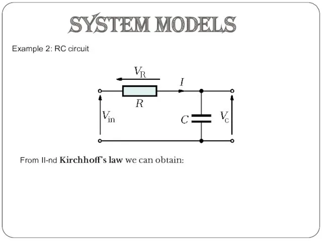
Example 2: RC circuit
System models
From II-nd Kirchhoff's law we can obtain:
Example 2: RC circuit
System models
From II-nd Kirchhoff's law we can obtain:
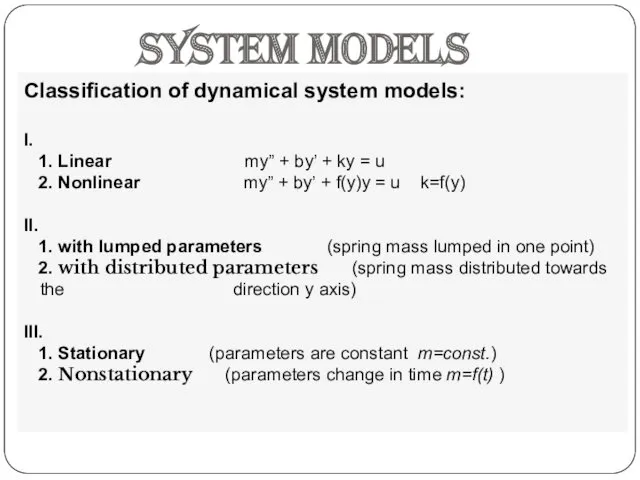
System models
Classification of dynamical system models:
I.
1. Linear my” + by’
System models
Classification of dynamical system models:
I.
1. Linear my” + by’
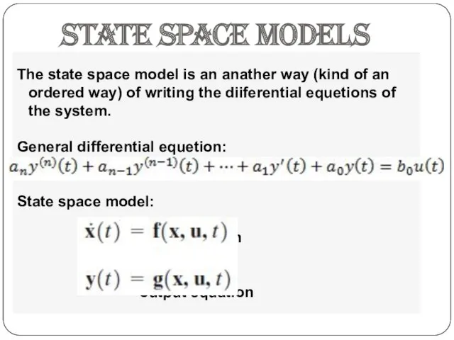
State space models
The state space model is an anather way (kind
State space models
The state space model is an anather way (kind
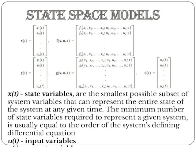
x(t) - state variables, are the smallest possible subset of system
x(t) - state variables, are the smallest possible subset of system
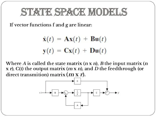
State space models
If vector functions f and g are linear:
Where
State space models
If vector functions f and g are linear:
Where
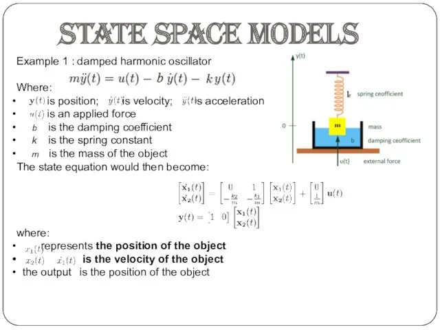
Example 1 : damped harmonic oscillator
Where:
is position; is velocity; is
Example 1 : damped harmonic oscillator
Where:
is position; is velocity; is
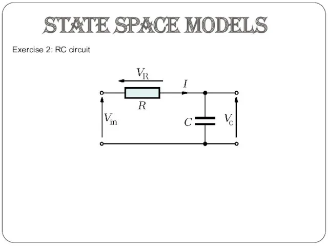
Exercise 2: RC circuit
State space models
Exercise 2: RC circuit
State space models
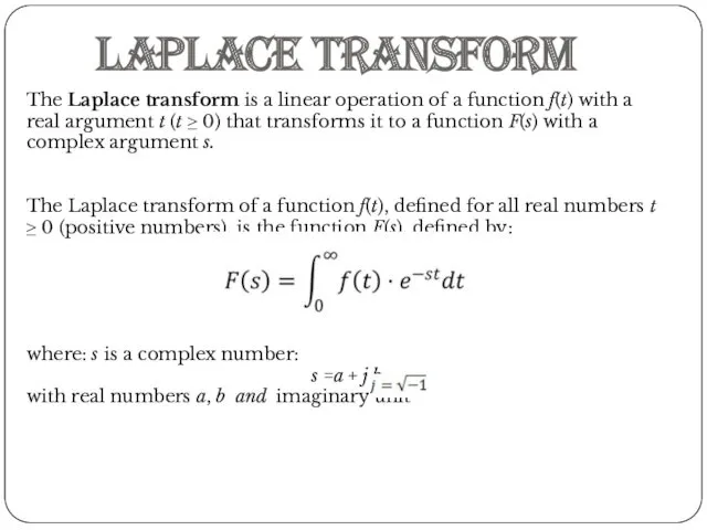
The Laplace transform is a linear operation of a function f(t)
The Laplace transform is a linear operation of a function f(t)
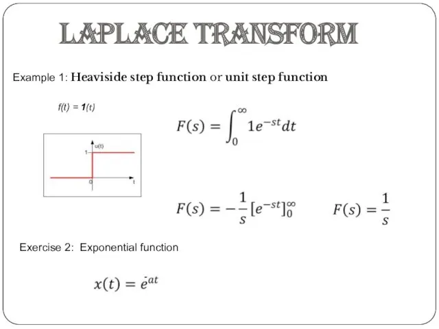
Example 1: Heaviside step function or unit step function
Laplace Transform
f(t) =
Example 1: Heaviside step function or unit step function
Laplace Transform
f(t) =
Laplace Transform
It is often convenient to use the differentiation property of
Laplace Transform
It is often convenient to use the differentiation property of
f(t) F(s)
Laplace Transform
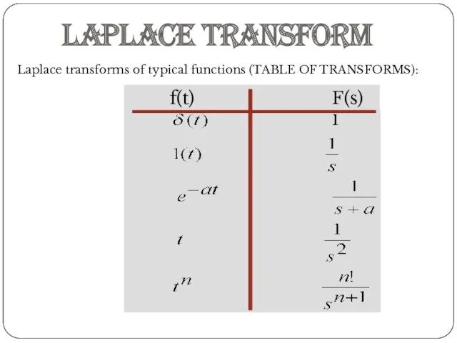
Laplace transforms of typical functions (TABLE OF TRANSFORMS):
f(t) F(s)
Laplace Transform
Laplace transforms of typical functions (TABLE OF TRANSFORMS):
Laplace Transform
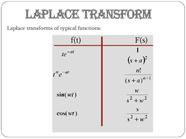
Laplace transforms of typical functions:
f(t) F(s)
Laplace Transform
Laplace transforms of typical functions:
f(t) F(s)
Laplace Transform
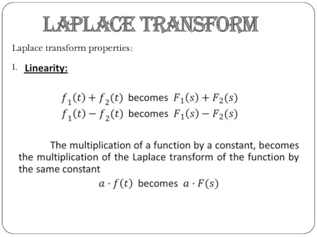
Laplace transform properties:
1.
Laplace Transform
Laplace transform properties:
1.
Laplace Transform
Laplace transform properties:
2.
becomes
Laplace Transform
Laplace transform properties:
2.
becomes
Laplace Transform
Laplace transform properties:
3.
4.
Laplace Transform
Laplace transform properties:
3.
4.
Laplace Transform
Laplace transform properties:
5.
6.
The final value theorem is useful because it
Laplace Transform
Laplace transform properties:
5.
6.
The final value theorem is useful because it
Inverse Laplace Transform
The Inverse Laplace Transform is defined by:
If the algebraic equation is
Inverse Laplace Transform
The Inverse Laplace Transform is defined by:
If the algebraic equation is
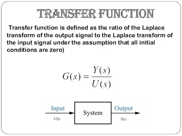
TRANSFER FUNCTION
Transfer function is defined as the ratio of the
TRANSFER FUNCTION
Transfer function is defined as the ratio of the
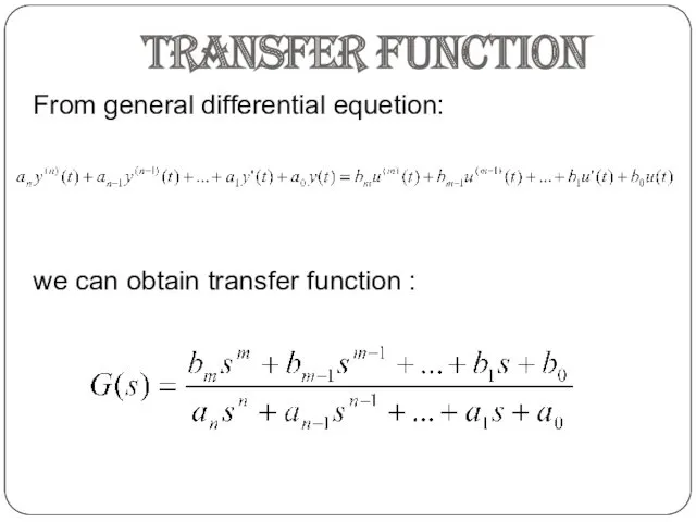
TRANSFER FUNCTION
From general differential equetion:
we can obtain transfer
TRANSFER FUNCTION
From general differential equetion:
we can obtain transfer
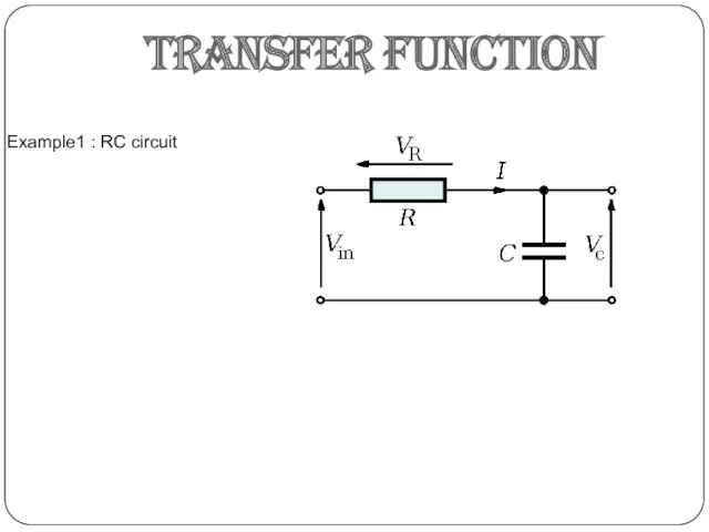
Example1 : RC circuit
TRANSFER FUNCTION
Example1 : RC circuit
TRANSFER FUNCTION
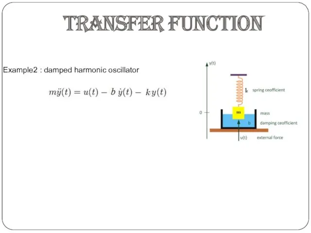
Example2 : damped harmonic oscillator
TRANSFER FUNCTION
Example2 : damped harmonic oscillator
TRANSFER FUNCTION
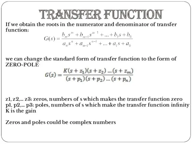
If we obtain the roots in the numerator and denominator of
If we obtain the roots in the numerator and denominator of
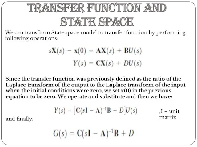
We can transform State space model to transfer function by performing
We can transform State space model to transfer function by performing
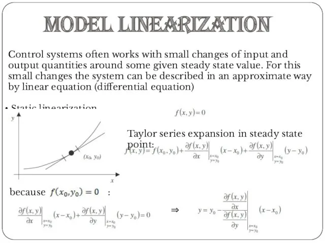
Control systems often works with small changes of input and output
Control systems often works with small changes of input and output
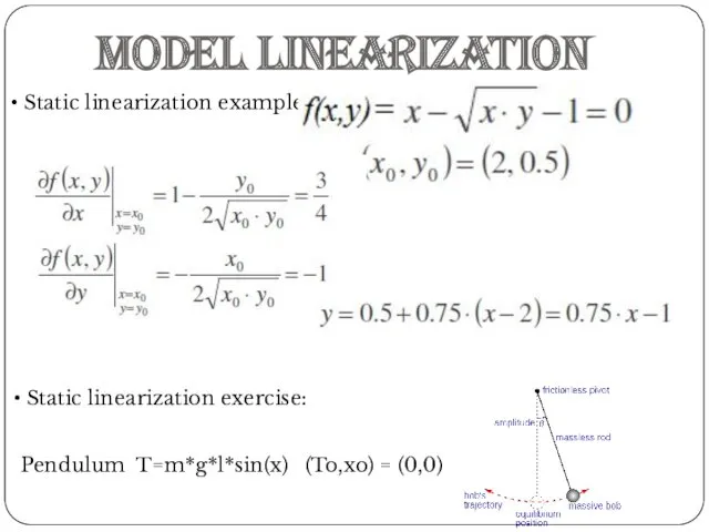
Static linearization example:
Model linearization
Static linearization exercise:
Pendulum
Static linearization example:
Model linearization
Static linearization exercise:
Pendulum
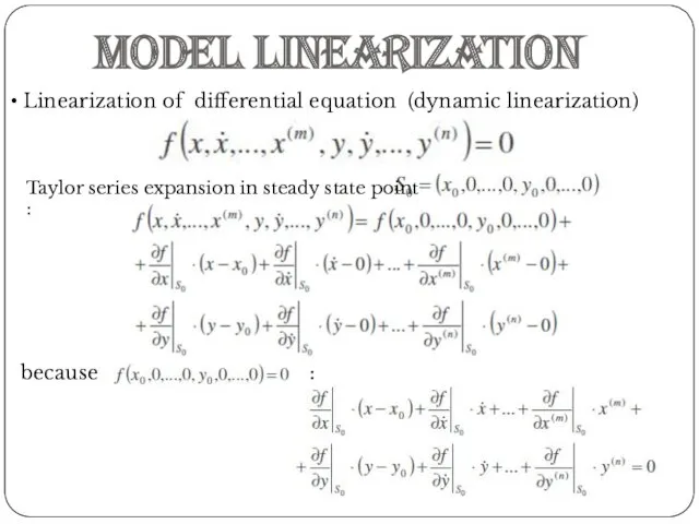
Linearization of differential equation (dynamic linearization)
Model linearization
Taylor series expansion
Linearization of differential equation (dynamic linearization)
Model linearization
Taylor series expansion
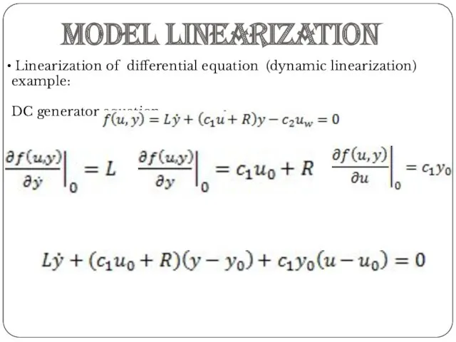
Linearization of differential equation (dynamic linearization) example:
DC generator equation:
Model
Linearization of differential equation (dynamic linearization) example:
DC generator equation:
Model

THANK YOU
THANK YOU
 Открытка к Дню защитника Отечества
 Свойства параллельных плоскостей
 Танцы народов Кавказа
 Разложение многочленов на множители
 презентация Фронтовая тетрадь- песенник Трифонова С.И.
 Развитие чувства времени у детей старшего дошкольного возраста
 Виды работы по воспитанию правильного произношения
 Отгадай слово по первым звукам
 Реформы в 1900 – 1912 гг
 Электрические трансформаторы. Расчет трансформаторов
 класс Вред
 Морфологический разбор имени существительного
 Инструктаж по ТБ и ОТ. Введение: инструктаж, знакомство
 Прсоединение Крыма к России
 Каменный век на Кавказе
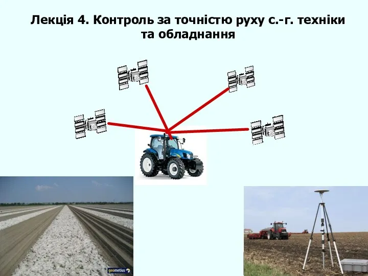 Контроль за точністю руху сільськогосподарської техніки та обладнання
 К. Паустовский Теплый хлеб
 Анализ работы фонда скважин Сологаевского месторождения пласта Д
 Мастер-класс Использование технологии развития критического мышления через чтение и письмо на примере урока чтения во 2 классе по теме В. Драгунский Заколдованная буква
 Microsoft Word. Создание первого документа Word
 практические работы
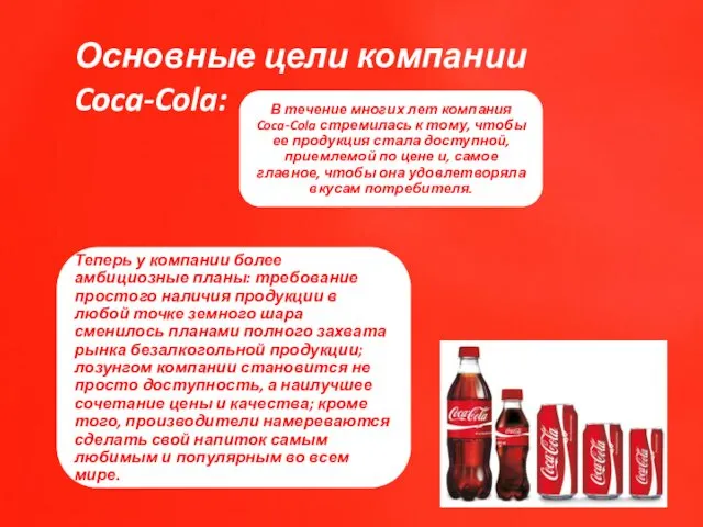 Цели компании Coca-Cola
 Презентация Дифференциация звуков Б-П
 مهارات الحاسب الآلي
 Презентация Петр Великий
 Авраам Линкольн
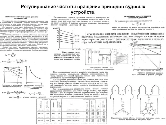 Регулирование частоты вращения приводов судовых устройств. Техническое обслуживание Дизель-генераторов. (Билет 30)
 Путешествие в космос