- The economic problem

Содержание
- 2. THE ECONOMIC PROBLEM 2
- 3. After studying this chapter, you will be able to: Define the production possibilities frontier and use
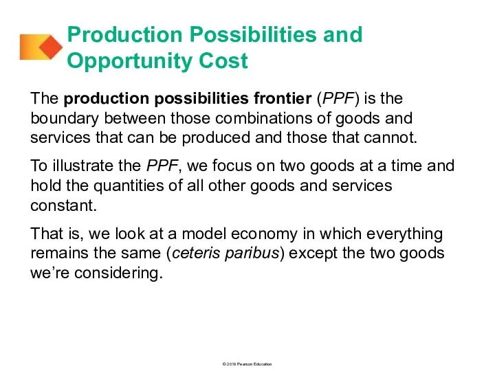
- 4. The production possibilities frontier (PPF) is the boundary between those combinations of goods and services that
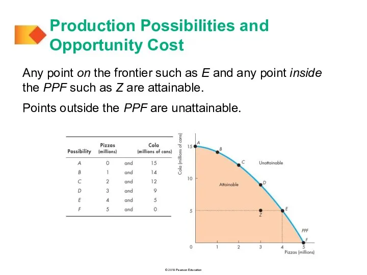
- 5. Production Possibilities Frontier Figure 2.1 shows the PPF for two goods: cola and pizzas. Production Possibilities
- 7. Any point on the frontier such as E and any point inside the PPF such as
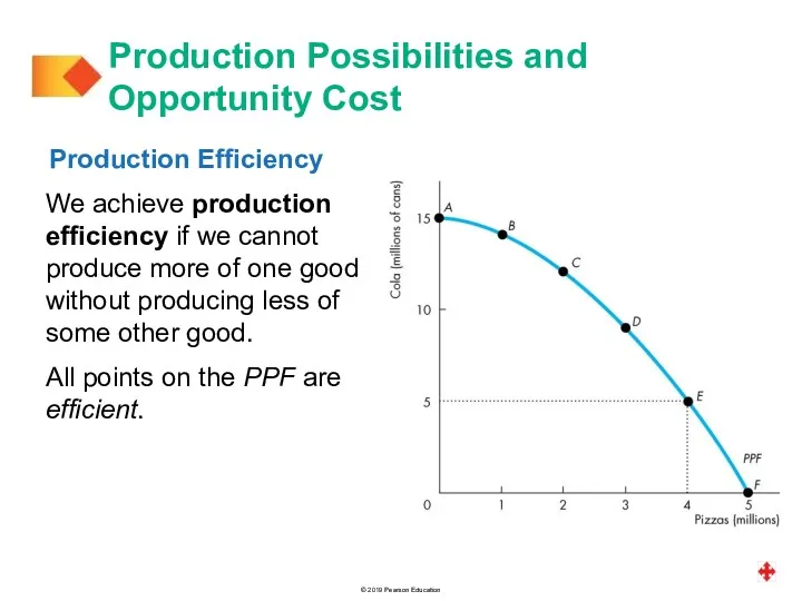
- 8. Production Efficiency We achieve production efficiency if we cannot produce more of one good without producing
- 10. Any point inside the frontier, such as Z, is inefficient. At such a point, it is
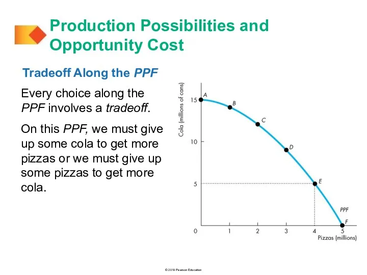
- 11. Tradeoff Along the PPF Every choice along the PPF involves a tradeoff. On this PPF, we
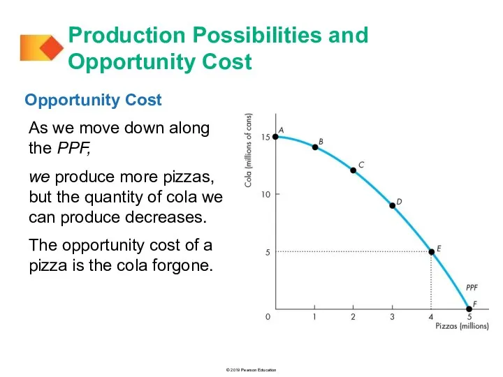
- 12. Opportunity Cost As we move down along the PPF, we produce more pizzas, but the quantity
- 13. In moving from E to F: The quantity of pizzas increases by 1 million. The quantity
- 14. In moving from F to E: The quantity of cola increases by 5 million cans. The
- 15. Opportunity Cost Is a Ratio The opportunity cost of producing a can of cola is the
- 16. Increasing Opportunity Cost Because resources are not equally productive in all activities, the PPF bows outward.
- 17. All the points along the PPF are efficient. To determine which of the alternative efficient quantities
- 18. Figure 2.2 illustrates the marginal cost of a pizza. As we move along the PPF, the
- 20. In part (b) of Fig. 2.2, the bars illustrate the increasing opportunity cost of a pizza.
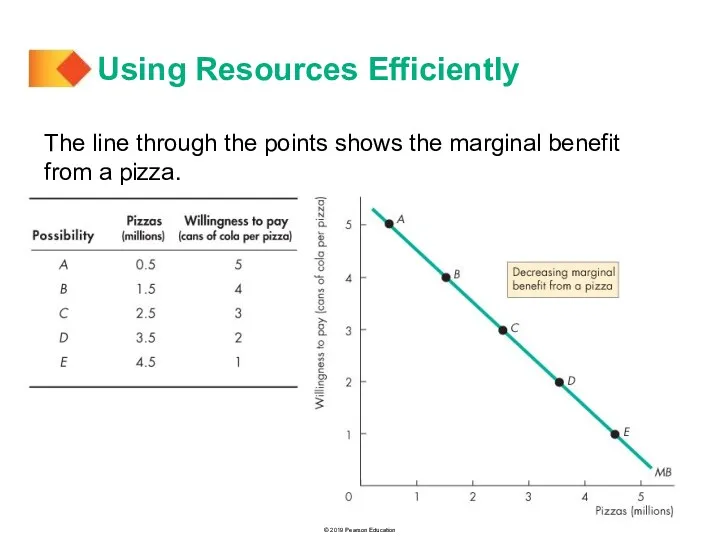
- 22. Preferences and Marginal Benefit Preferences are a description of a person’s likes and dislikes. To describe
- 23. It is a general principle that: The more we have of any good, the smaller is
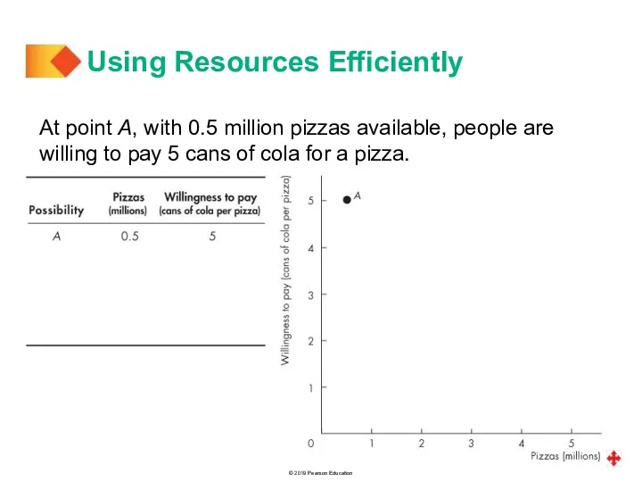
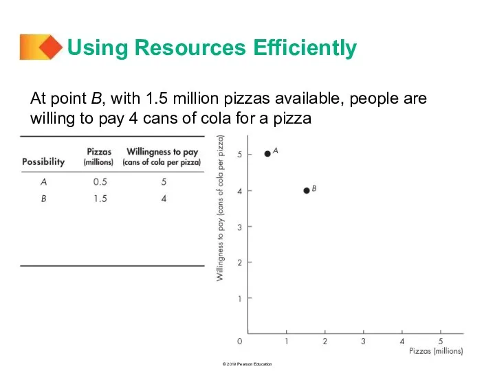
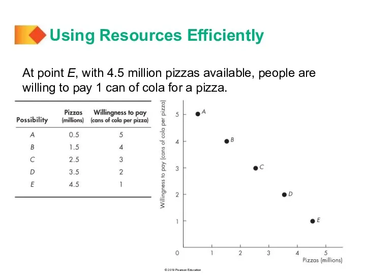
- 24. At point A, with 0.5 million pizzas available, people are willing to pay 5 cans of
- 26. At point B, with 1.5 million pizzas available, people are willing to pay 4 cans of
- 27. At point E, with 4.5 million pizzas available, people are willing to pay 1 can of
- 28. The line through the points shows the marginal benefit from a pizza. Using Resources Efficiently
- 29. Allocative Efficiency When we cannot produce more of any one good without giving up some other
- 30. Figure 2.4 illustrates allocative efficiency. The point of allocative efficiency is the point on the PPF
- 32. If we produce 1.5 million pizzas, marginal benefit exceeds marginal cost. We get more value from
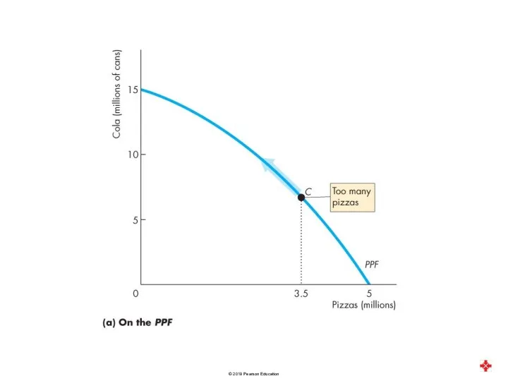
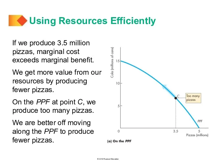
- 33. If we produce 3.5 million pizzas, marginal cost exceeds marginal benefit. We get more value from
- 34. On the PPF at point B, we are producing the efficient quantities of pizzas and cola.
- 36. Comparative Advantage and Absolute Advantage A person has a comparative advantage in an activity if that
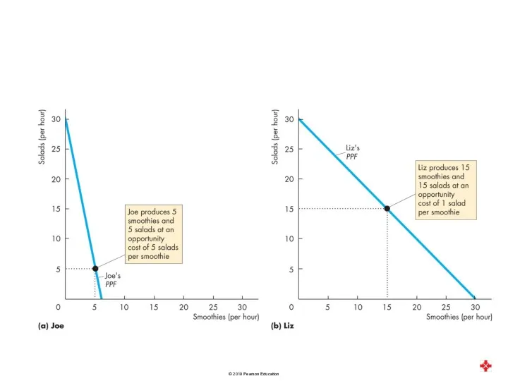
- 37. Joe’s Smoothie Bar In an hour, Joe can produce 6 smoothies or 30 salads. Joe's opportunity
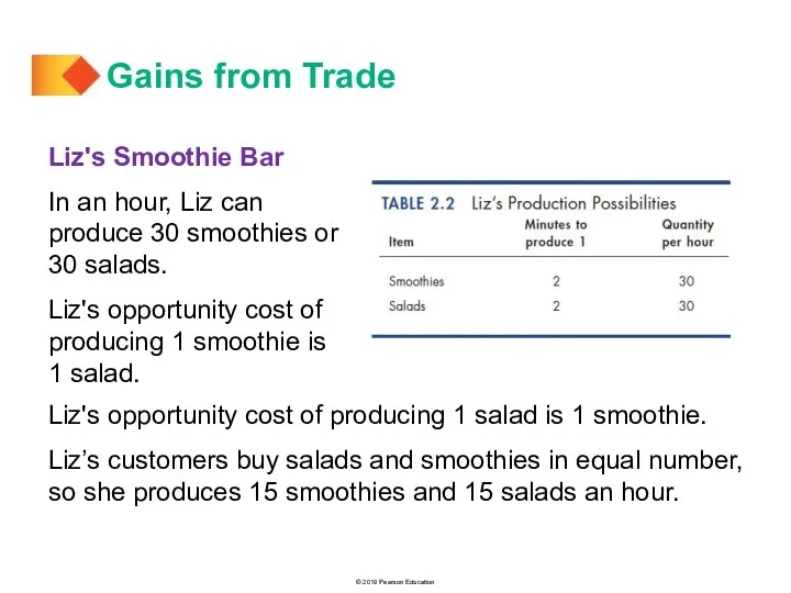
- 38. Liz's opportunity cost of producing 1 salad is 1 smoothie. Liz’s customers buy salads and smoothies
- 39. Figure 2.5 shows the production possibility frontiers. In part (a), Joe’s opportunity cost of a smoothie
- 41. In part (b), Liz’s opportunity cost of a smoothie is 1 salad. Liz produces at point
- 42. Joe’s Comparative Advantage Joe’s opportunity cost of a salad is 1/5 smoothie. Liz’s opportunity cost of
- 43. Liz’s Comparative Advantage Liz’s opportunity cost of a smoothie is 1 salad. Joe’s opportunity cost of
- 44. Achieving the Gains from Trade Liz and Joe produce the good in which they have a
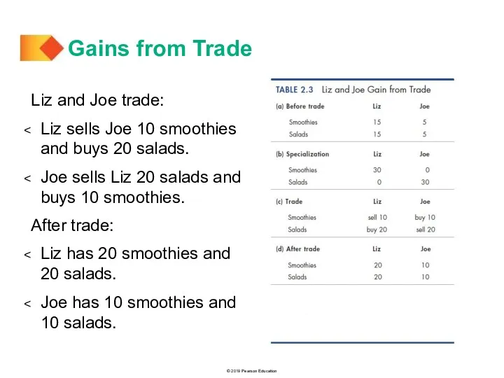
- 46. Liz and Joe trade: Liz sells Joe 10 smoothies and buys 20 salads. Joe sells Liz
- 47. Gains from trade: Liz gains 5 smoothies and 5 salads an hour Joe gains 5 smoothies
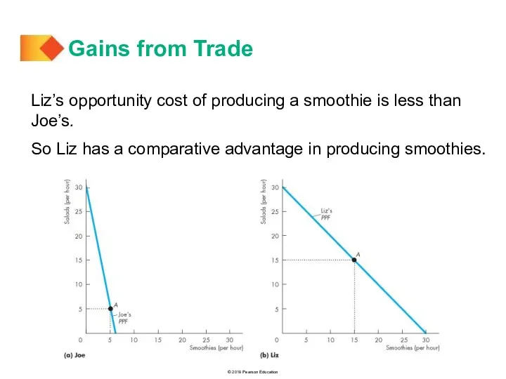
- 48. Figure 2.6 shows the gains from trade. Joe’s opportunity cost of producing a salad is less
- 50. Liz’s opportunity cost of producing a smoothie is less than Joe’s. So Liz has a comparative
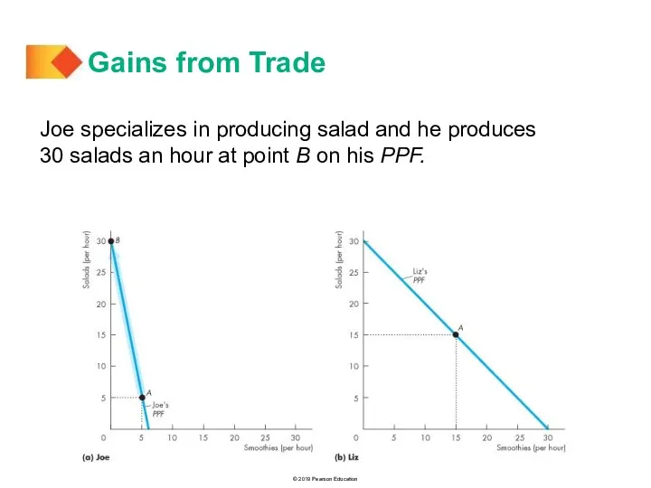
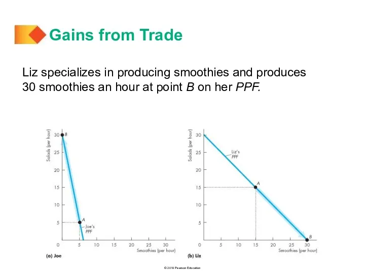
- 51. Joe specializes in producing salad and he produces 30 salads an hour at point B on
- 52. Liz specializes in producing smoothies and produces 30 smoothies an hour at point B on her
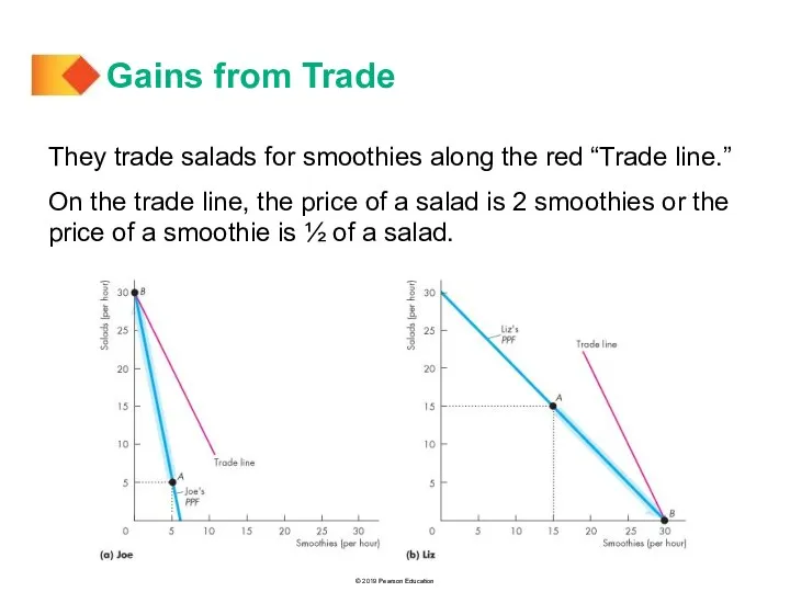
- 53. They trade salads for smoothies along the red “Trade line.” On the trade line, the price
- 54. Joe buys smoothies from Liz and moves to point C—a point outside his PPF. Liz buys
- 55. The Liz-Joe Economy and its PPF With specialization and trade both Liz and Joe get outside
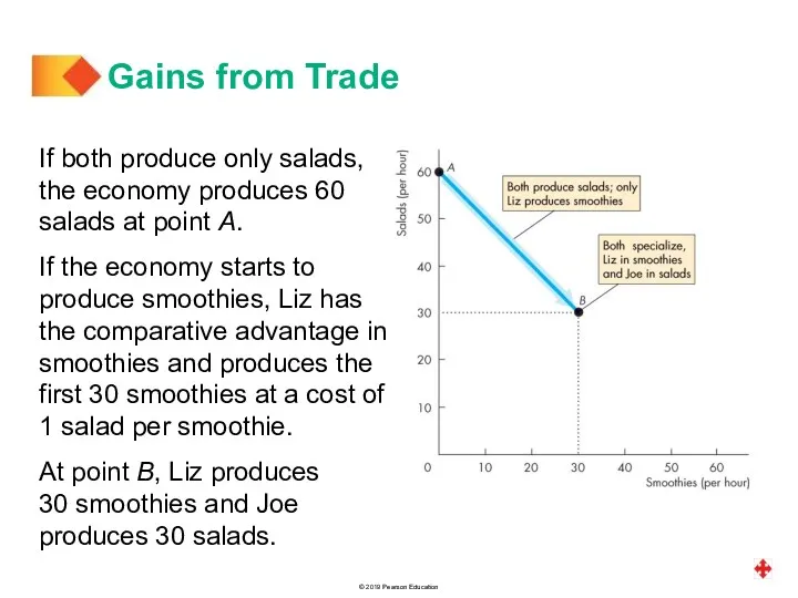
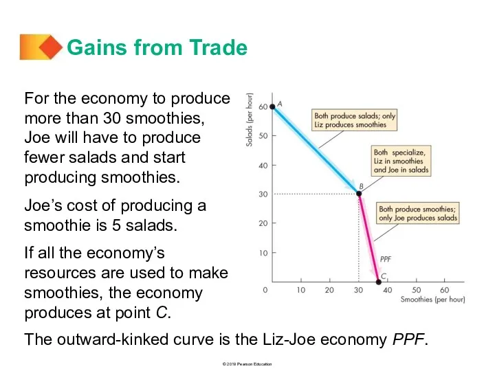
- 56. If both produce only salads, the economy produces 60 salads at point A. If the economy
- 58. For the economy to produce more than 30 smoothies, Joe will have to produce fewer salads
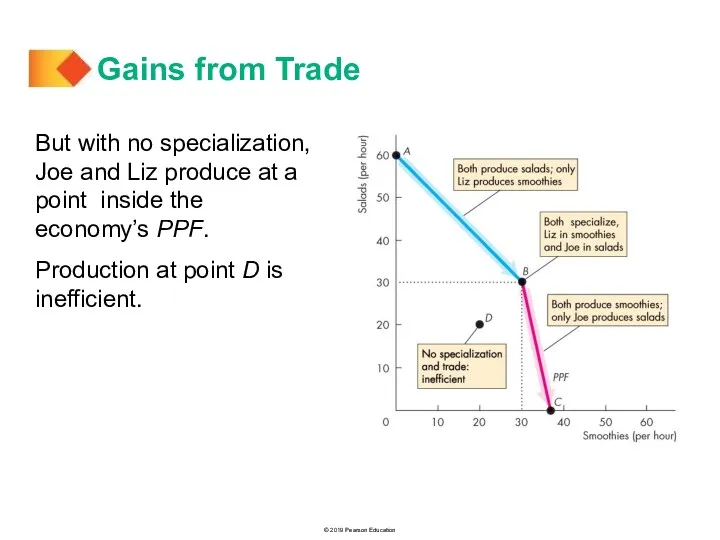
- 59. Efficiency and Inefficiency When both Liz and Joe specialize, they produce efficiently at point B on
- 60. But with no specialization, Joe and Liz produce at a point inside the economy’s PPF. Production
- 61. The expansion of production possibilities—an increase in the standard of living—is called economic growth. Two key
- 62. The Cost of Economic Growth To use resources in research and development and to produce new
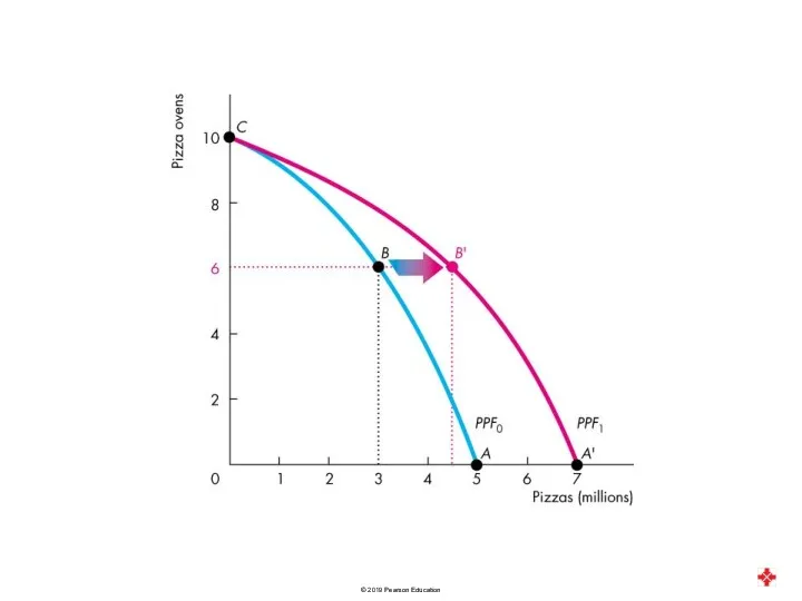
- 63. Figure 2.8 illustrates the tradeoff we face. We can produce pizzas or pizza ovens along PPF0.
- 65. Changes in What We Produce Investment in capital and technology creates economic growth and increases income.
- 66. Figure 2.9(a) compares low-income Ethiopia and China. Figure 2.9(b) compares China and the rich United States.
- 68. To reap the gains from trade, the choices of individuals must be coordinated. To make coordination
- 69. A firm is an economic unit that hires factors of production and organizes those factors to
- 70. Economic Coordination Circular Flows Through Markets Figure 2.8 illustrates how households and firms interact in the
- 73. Скачать презентацию
THE ECONOMIC PROBLEM
2
THE ECONOMIC PROBLEM
2
After studying this chapter, you will be able to:
Define the production
After studying this chapter, you will be able to:
Define the production
The production possibilities frontier (PPF) is the boundary between those combinations
The production possibilities frontier (PPF) is the boundary between those combinations

Production Possibilities Frontier
Figure 2.1 shows the PPF for two goods: cola
Production Possibilities Frontier
Figure 2.1 shows the PPF for two goods: cola

Any point on the frontier such as E and any point
Any point on the frontier such as E and any point
Production Efficiency
We achieve production efficiency if we cannot produce more of
Production Efficiency
We achieve production efficiency if we cannot produce more of

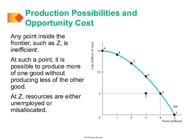
Any point inside the frontier, such as Z, is inefficient.
At such
Any point inside the frontier, such as Z, is inefficient.
At such
Tradeoff Along the PPF
Every choice along the PPF involves a tradeoff.
On
Tradeoff Along the PPF
Every choice along the PPF involves a tradeoff.
On
Opportunity Cost
As we move down along the PPF,
we produce more
Opportunity Cost
As we move down along the PPF,
we produce more

In moving from E to F:
The quantity of pizzas increases by
In moving from E to F:
The quantity of pizzas increases by

In moving from F to E:
The quantity of cola increases by
In moving from F to E:
The quantity of cola increases by

Opportunity Cost Is a Ratio
The opportunity cost of producing a
Opportunity Cost Is a Ratio
The opportunity cost of producing a
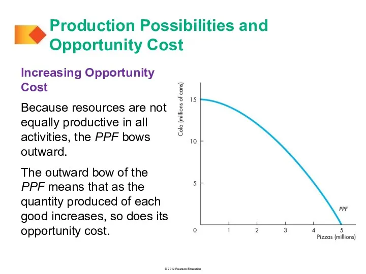
Increasing Opportunity Cost
Because resources are not equally productive in all activities,
Increasing Opportunity Cost
Because resources are not equally productive in all activities,
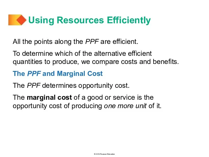
All the points along the PPF are efficient.
To determine which of
All the points along the PPF are efficient.
To determine which of
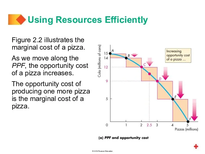
Figure 2.2 illustrates the marginal cost of a pizza.
As we move
Figure 2.2 illustrates the marginal cost of a pizza.
As we move


In part (b) of Fig. 2.2, the bars illustrate the increasing
In part (b) of Fig. 2.2, the bars illustrate the increasing

Preferences and Marginal Benefit
Preferences are a description of a person’s likes
Preferences and Marginal Benefit
Preferences are a description of a person’s likes
It is a general principle that:
The more we have of any
It is a general principle that:
The more we have of any
At point A, with 0.5 million pizzas available, people are willing
At point A, with 0.5 million pizzas available, people are willing

At point B, with 1.5 million pizzas available, people are willing
At point B, with 1.5 million pizzas available, people are willing
At point E, with 4.5 million pizzas available, people are willing
At point E, with 4.5 million pizzas available, people are willing
The line through the points shows the marginal benefit from a
The line through the points shows the marginal benefit from a

Allocative Efficiency
When we cannot produce more of any one good without
Allocative Efficiency
When we cannot produce more of any one good without

Figure 2.4 illustrates allocative efficiency.
The point of allocative efficiency is the
Figure 2.4 illustrates allocative efficiency.
The point of allocative efficiency is the

If we produce 1.5 million pizzas, marginal benefit exceeds marginal cost.
We
If we produce 1.5 million pizzas, marginal benefit exceeds marginal cost.
We
If we produce 3.5 million pizzas, marginal cost exceeds marginal benefit.
We
If we produce 3.5 million pizzas, marginal cost exceeds marginal benefit.
We

On the PPF at point B, we are producing the efficient
On the PPF at point B, we are producing the efficient


Comparative Advantage and Absolute Advantage
A person has a comparative advantage in
Comparative Advantage and Absolute Advantage
A person has a comparative advantage in

Joe’s Smoothie Bar
In an hour, Joe can produce 6 smoothies or
Joe’s Smoothie Bar
In an hour, Joe can produce 6 smoothies or
Liz's opportunity cost of producing 1 salad is 1 smoothie.
Liz’s
Liz's opportunity cost of producing 1 salad is 1 smoothie.
Liz’s

Figure 2.5 shows the production possibility frontiers.
In part (a), Joe’s opportunity
Figure 2.5 shows the production possibility frontiers.
In part (a), Joe’s opportunity

In part (b), Liz’s opportunity cost of a smoothie is 1
In part (b), Liz’s opportunity cost of a smoothie is 1
Joe’s Comparative Advantage
Joe’s opportunity cost of a salad is 1/5 smoothie.
Liz’s
Joe’s Comparative Advantage
Joe’s opportunity cost of a salad is 1/5 smoothie.
Liz’s
Liz’s Comparative Advantage
Liz’s opportunity cost of a smoothie is 1 salad.
Joe’s
Liz’s Comparative Advantage
Liz’s opportunity cost of a smoothie is 1 salad.
Joe’s
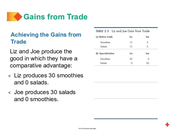
Achieving the Gains from Trade
Liz and Joe produce the good in
Achieving the Gains from Trade
Liz and Joe produce the good in

Liz and Joe trade:
Liz sells Joe 10 smoothies and buys 20
Liz and Joe trade:
Liz sells Joe 10 smoothies and buys 20
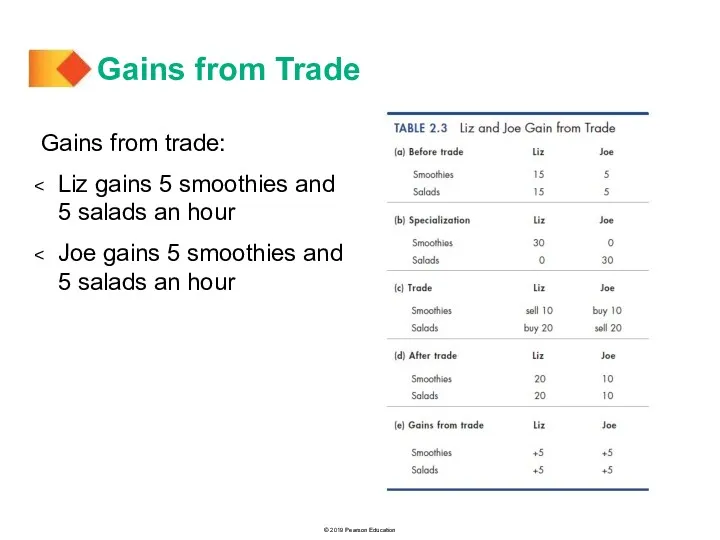
Gains from trade:
Liz gains 5 smoothies and
5 salads an hour
Joe
Gains from trade:
Liz gains 5 smoothies and
5 salads an hour
Joe

Figure 2.6 shows the gains from trade.
Joe’s opportunity cost of producing
Figure 2.6 shows the gains from trade.
Joe’s opportunity cost of producing

Liz’s opportunity cost of producing a smoothie is less than Joe’s.
So
Liz’s opportunity cost of producing a smoothie is less than Joe’s.
So
Joe specializes in producing salad and he produces
30 salads an
Joe specializes in producing salad and he produces 30 salads an
Liz specializes in producing smoothies and produces
30 smoothies an hour
Liz specializes in producing smoothies and produces 30 smoothies an hour
They trade salads for smoothies along the red “Trade line.”
On
They trade salads for smoothies along the red “Trade line.”
On

Joe buys smoothies from Liz and moves to point C—a point
Joe buys smoothies from Liz and moves to point C—a point
The Liz-Joe Economy and its PPF
With specialization and trade both Liz
The Liz-Joe Economy and its PPF
With specialization and trade both Liz
If both produce only salads, the economy produces 60 salads at
If both produce only salads, the economy produces 60 salads at

For the economy to produce more than 30 smoothies, Joe will
For the economy to produce more than 30 smoothies, Joe will

Efficiency and Inefficiency
When both Liz and Joe specialize, they produce efficiently
Efficiency and Inefficiency
When both Liz and Joe specialize, they produce efficiently
But with no specialization, Joe and Liz produce at a point
But with no specialization, Joe and Liz produce at a point
The expansion of production possibilities—an increase in the standard of living—is
The expansion of production possibilities—an increase in the standard of living—is
The Cost of Economic Growth
To use resources in research and development
The Cost of Economic Growth
To use resources in research and development
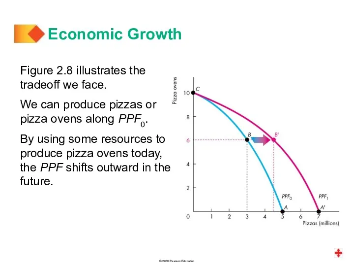
Figure 2.8 illustrates the tradeoff we face.
We can produce pizzas or
Figure 2.8 illustrates the tradeoff we face.
We can produce pizzas or

Changes in What We Produce
Investment in capital and technology creates economic
Changes in What We Produce
Investment in capital and technology creates economic
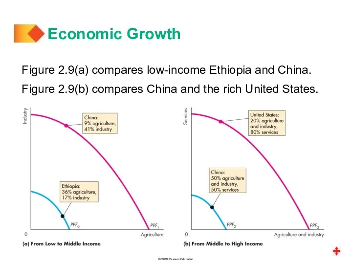
Figure 2.9(a) compares low-income Ethiopia and China.
Figure 2.9(b) compares China and
Figure 2.9(a) compares low-income Ethiopia and China.
Figure 2.9(b) compares China and


To reap the gains from trade, the choices of individuals must
To reap the gains from trade, the choices of individuals must

A firm is an economic unit that hires factors of production
A firm is an economic unit that hires factors of production

Economic Coordination
Circular Flows
Through Markets
Figure 2.8 illustrates how households and firms
Economic Coordination
Circular Flows
Through Markets
Figure 2.8 illustrates how households and firms

 Экономикалық талдаудың әдістері мен тәсілдері
 Экономика предприятий и организаций
 Структурная политика
 Анализ рыночных структур. Модель совершенной конкуренции
 Подготовка и организация производственной деятельности
 Инвестирование – основа расширенного воспроизводства
 Отчёт о результатах деятельности главы и администрации городского округа Новокуйбышевск
 Государственное макроэкономическое регулирование. Социальная политика государства. Международные аспекты макроэкономики
 Экономические стратегии в домохозяйстве на примере конкретных стран
 Об организации информационного статистического обеспечения мониторинга реализации задач, установленных в указе президента РФ
 Правове регулювання ринку зерна в Україні
 Предмет и методы экономической географии и регионалистики
 Демографическая ситуация в современной России
 Сетевые организации
 Доход за вычетом издержек
 Introduction to Investments (Chapter 1)
 Экономические циклы. Лекция 8
 Основные производственные фонды
 Причины образования потерь
 Макроэкономикалық көрсеткіш
 Фактори виробництва
 Индонезия. Экономика Индонезии
 Supply and demand. Demand. Law of demand
 Мировая экономика и международное разделение труда
 Показники функціонування економічної системи
 Роль государства в экономике
 Безработица и занятость населения
 Основные макроэкономические показатели