- Synthetic-Aperture Radar (SAR) Image Formation Processing

Содержание
- 2. Outline Raw SAR image characteristics Algorithm basics Range compression Range cell migration correction Azimuth compression Motion
- 3. Airborne SAR real-time IFP block diagram Image-Formation Processor New terminology: Presum (a.k.a. coherent integration) Corner-turning memory
- 4. Basic SAR image formation processes
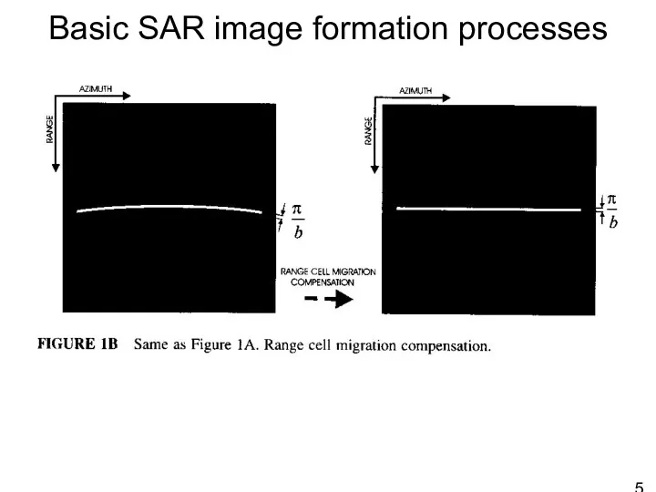
- 5. Basic SAR image formation processes
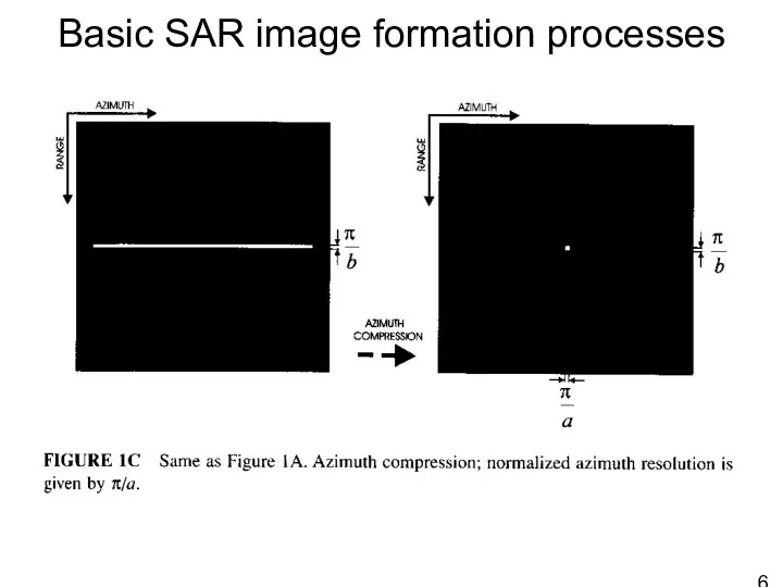
- 6. Basic SAR image formation processes
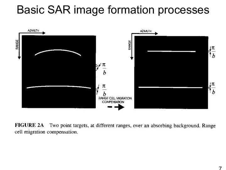
- 7. Basic SAR image formation processes
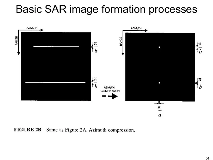
- 8. Basic SAR image formation processes
- 9. Optical image-formation processing
- 10. Demodulated baseband SAR signal [from Digital processing of synthetic aperture radar data, by Cumming and Wong,
- 11. Demodulated baseband SAR signal includes R-4 and target RCS factors Vr : effective radar velocity (a
- 12. SAR signal spectrum [from Digital processing of synthetic aperture radar data, by Cumming and Wong, 2005]
- 13. SAR signal spectrum Also fτ : range frequency, Hz, where –Fr /2 ≤ fτ ≤ Fr
- 14. SAR signal spectrum envelope of the radar data’s range spectrum antenna’s beam pattern envelope in Doppler
- 15. Matched filter processing Given an understanding of the characteristics of the ideal SAR signal, an ideal
- 16. Range Doppler domain spectrum [from Digital processing of synthetic aperture radar data, by Cumming and Wong,
- 17. Range migration
- 18. Range-dependent range migration Baz : azimuth bandwidth Br : transmitted pulse bandwidth ηo : azimuth time
- 19. Range-Doppler processing
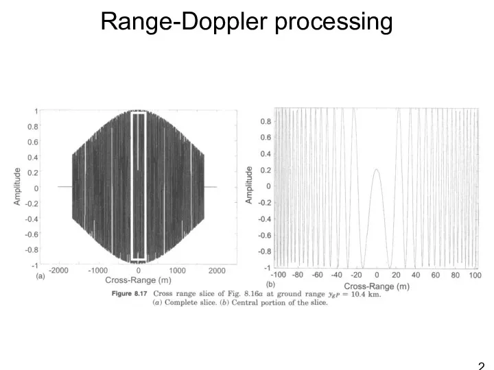
- 20. Range-Doppler processing
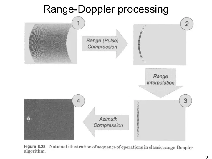
- 21. Range-Doppler processing
- 22. Range-Doppler algorithm RCMC: range cell migration compensation SRC: secondary range compression Range cell migration compensation (RCMC)
- 23. Range-cell migration compensation Part of the migration compensation requires a re-sampling of the range-compressed pulse using
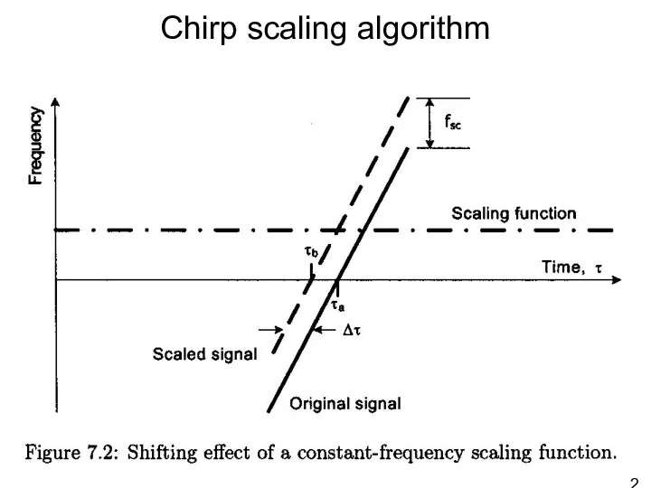
- 24. Chirp scaling algorithm The range-Doppler algorithm was the first digital algorithm developed for civilian satellite SAR
- 25. Chirp scaling algorithm
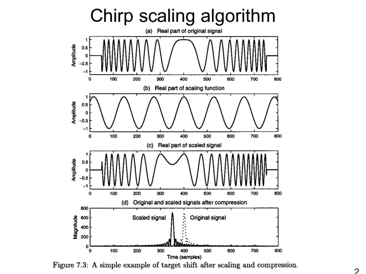
- 26. Chirp scaling algorithm
- 27. Chirp scaling algorithm
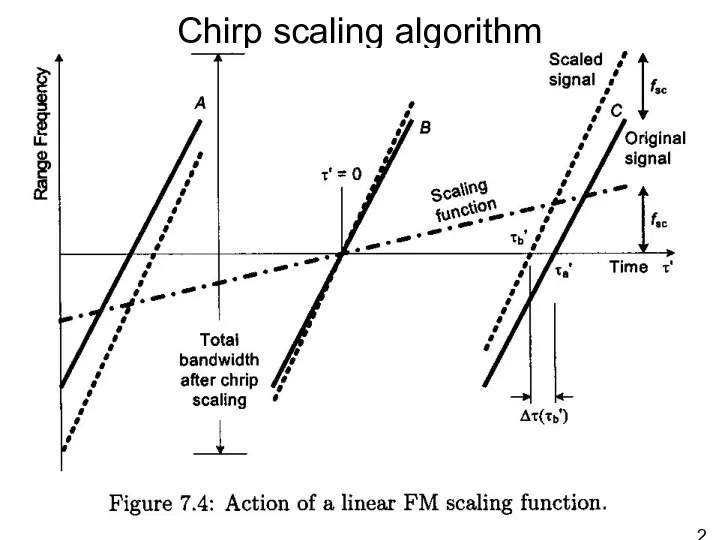
- 28. Chirp scaling algorithm
- 29. Chirp scaling algorithm
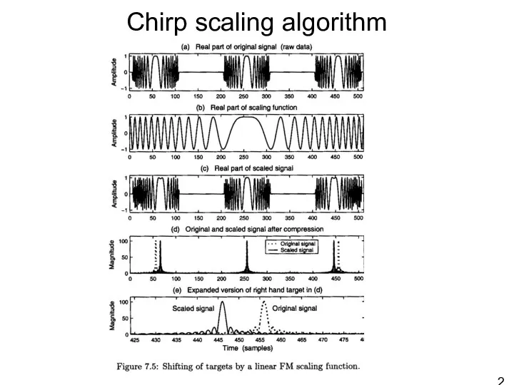
- 30. Range-cell migration compensation
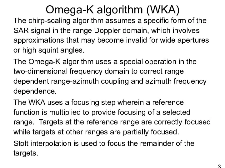
- 31. Omega-K algorithm (WKA) The chirp-scaling algorithm assumes a specific form of the SAR signal in the
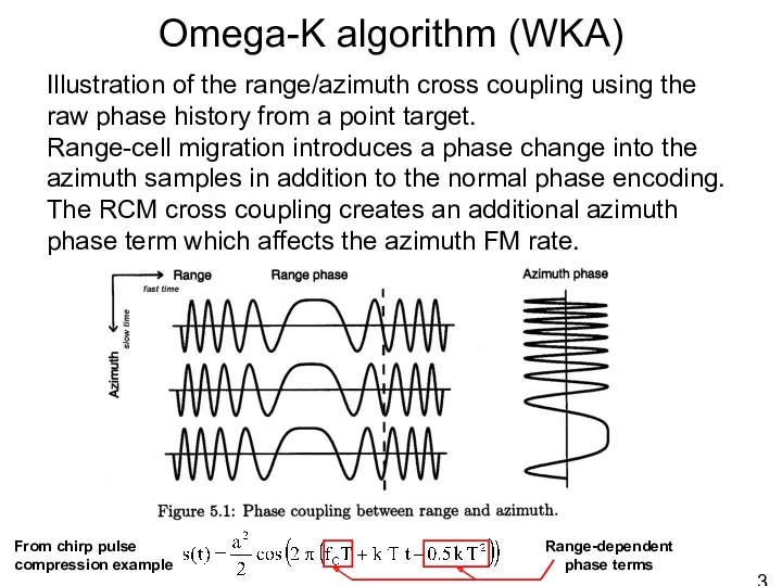
- 32. Omega-K algorithm (WKA) Illustration of the range/azimuth cross coupling using the raw phase history from a
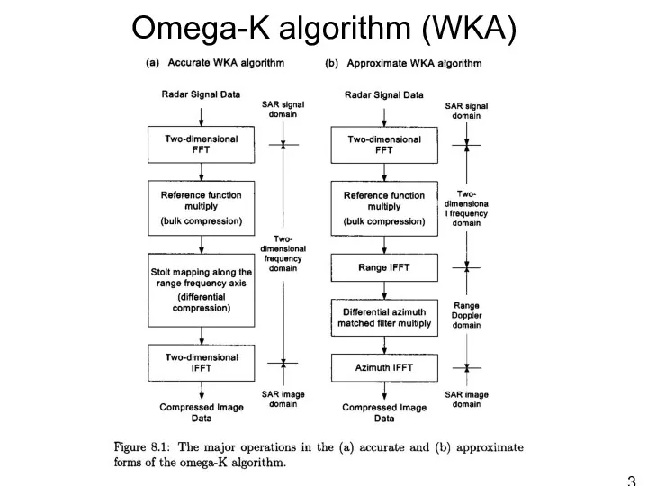
- 33. Omega-K algorithm (WKA)
- 34. Stolt interpolation
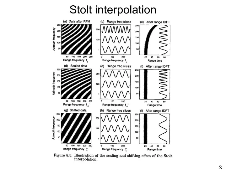
- 35. Stolt interpolation
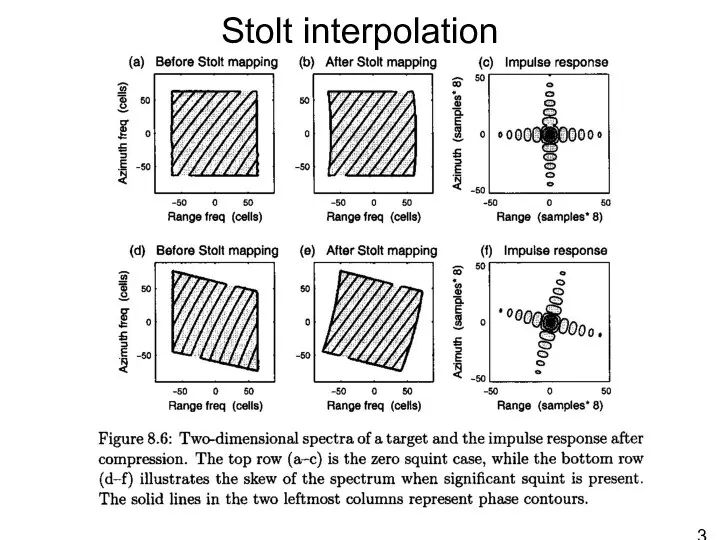
- 36. Stolt interpolation
- 37. Comparison of IFP algorithms Azim MF: azimuth matched filter Hyperb: hyperbolic P.S.: power series, i.e., parabolic
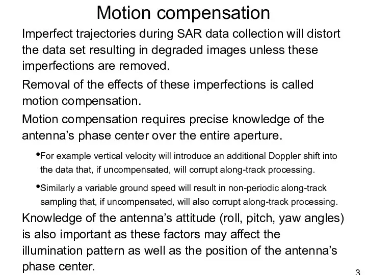
- 38. Motion compensation Imperfect trajectories during SAR data collection will distort the data set resulting in degraded
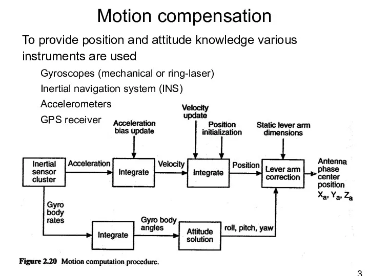
- 39. Motion compensation To provide position and attitude knowledge various instruments are used Gyroscopes (mechanical or ring-laser)
- 40. Motion compensation
- 41. Motion compensation In addition to position and attitude knowledge acquired from various external sensors and systems,
- 42. Autofocus Just as non-ideal motion corrupts the SAR’s phase history, the received signal can also reveal
- 43. Quadratic phase errors
- 44. High-frequency phase errors
- 45. Autofocus – inverse filtering
- 46. Autofocus – inverse filtering
- 47. Autofocus – phase gradient The phase gradient autofocus algorithm is unique in that it is not
- 49. Скачать презентацию
Outline
Raw SAR image characteristics
Algorithm basics
Range compression
Range cell migration correction
Azimuth compression
Motion compensation
Types
Outline
Raw SAR image characteristics
Algorithm basics
Range compression
Range cell migration correction
Azimuth compression
Motion compensation
Types
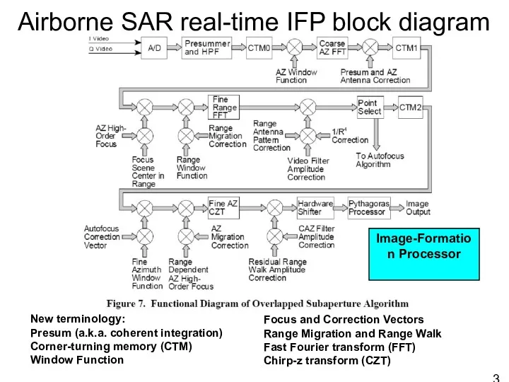
Airborne SAR real-time IFP block diagram
Image-Formation Processor
New terminology:
Presum (a.k.a. coherent integration)
Corner-turning
Airborne SAR real-time IFP block diagram
Image-Formation Processor
New terminology: Presum (a.k.a. coherent integration) Corner-turning
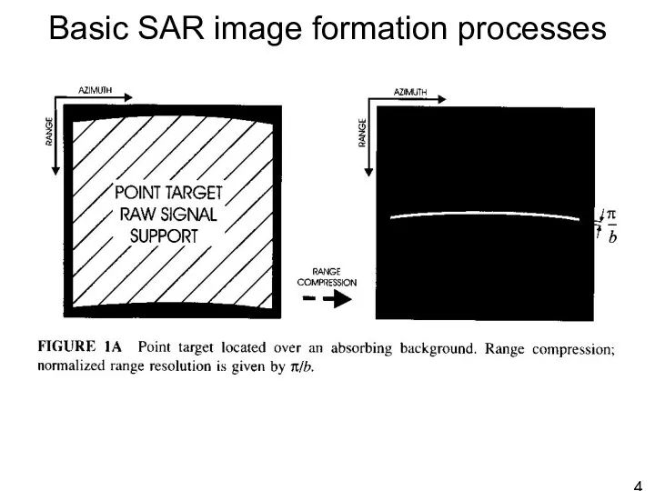
Basic SAR image formation processes
Basic SAR image formation processes
Basic SAR image formation processes
Basic SAR image formation processes
Basic SAR image formation processes
Basic SAR image formation processes
Basic SAR image formation processes
Basic SAR image formation processes
Basic SAR image formation processes
Basic SAR image formation processes
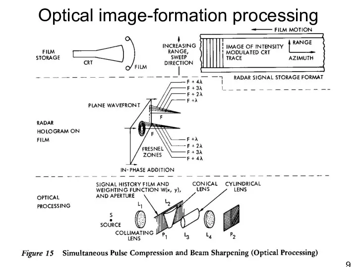
Optical image-formation processing
Optical image-formation processing
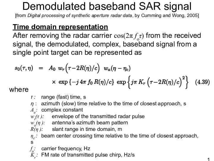
Demodulated baseband SAR signal
[from Digital processing of synthetic aperture radar data,
Demodulated baseband SAR signal [from Digital processing of synthetic aperture radar data,
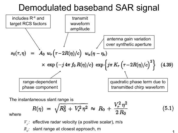
Demodulated baseband SAR signal
includes R-4 and target RCS factors
Vr : effective radar
Demodulated baseband SAR signal
includes R-4 and target RCS factors
Vr : effective radar
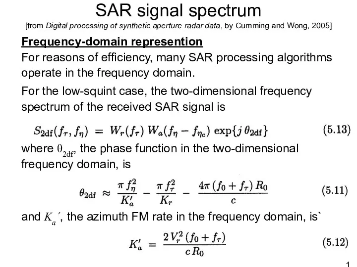
SAR signal spectrum
[from Digital processing of synthetic aperture radar data, by
SAR signal spectrum [from Digital processing of synthetic aperture radar data, by
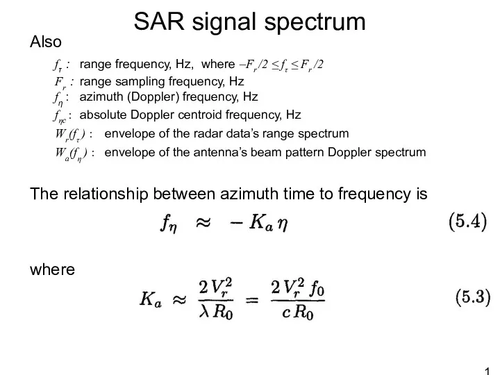
SAR signal spectrum
Also
fτ : range frequency, Hz, where –Fr /2 ≤ fτ
SAR signal spectrum
Also
fτ : range frequency, Hz, where –Fr /2 ≤ fτ
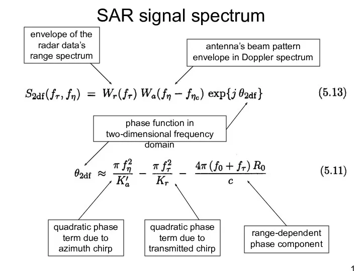
SAR signal spectrum
envelope of the radar data’s range spectrum
antenna’s beam pattern
SAR signal spectrum
envelope of the radar data’s range spectrum
antenna’s beam pattern
Matched filter processing
Given an understanding of the characteristics of the ideal
Matched filter processing
Given an understanding of the characteristics of the ideal
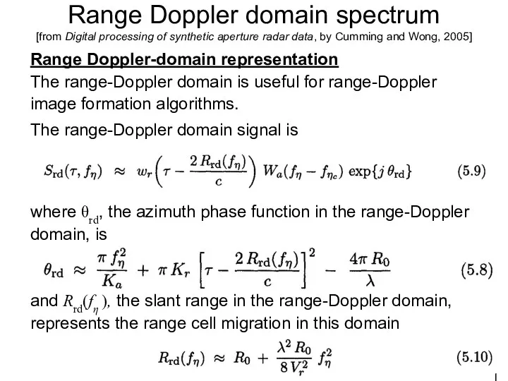
Range Doppler domain spectrum
[from Digital processing of synthetic aperture radar data,
Range Doppler domain spectrum [from Digital processing of synthetic aperture radar data,
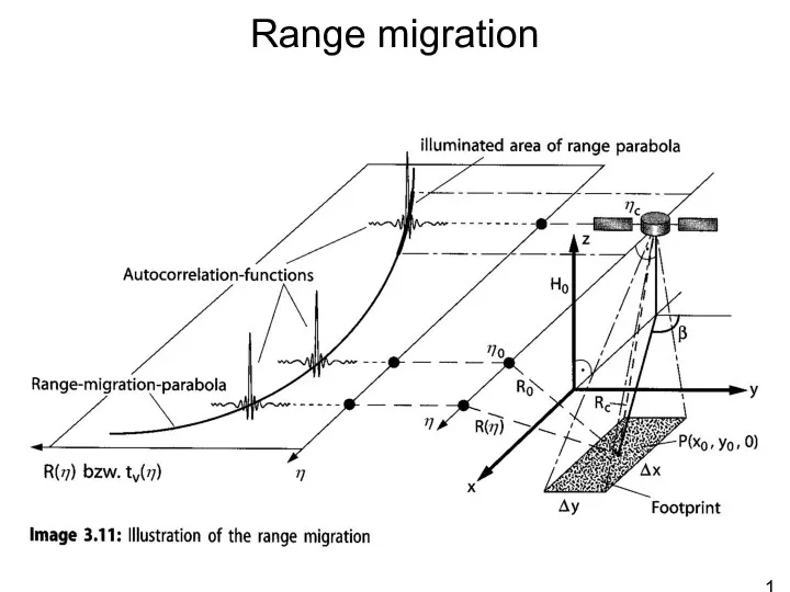
Range migration
Range migration
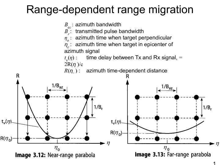
Range-dependent range migration
Baz : azimuth bandwidth
Br : transmitted pulse bandwidth
ηo : azimuth time when
Range-dependent range migration
Baz : azimuth bandwidth
Br : transmitted pulse bandwidth
ηo : azimuth time when
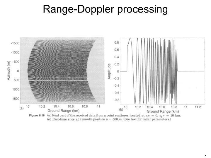
Range-Doppler processing
Range-Doppler processing
Range-Doppler processing
Range-Doppler processing
Range-Doppler processing
Range-Doppler processing
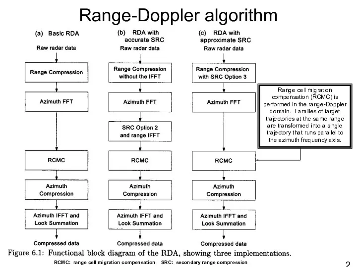
Range-Doppler algorithm
RCMC: range cell migration compensation SRC: secondary range compression
Range cell migration
Range-Doppler algorithm
RCMC: range cell migration compensation SRC: secondary range compression
Range cell migration
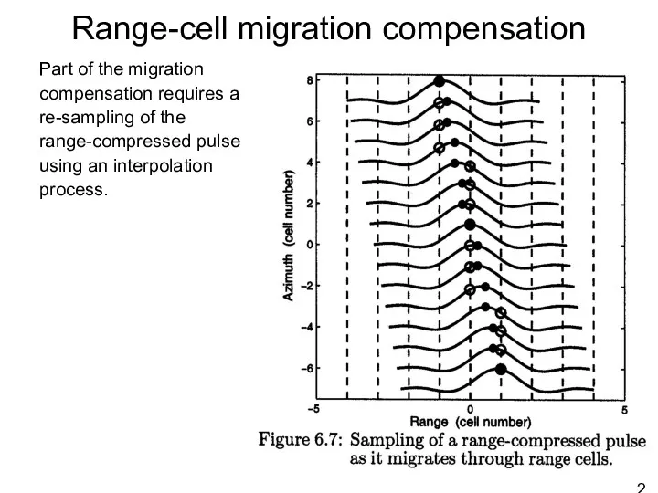
Range-cell migration compensation
Part of the migration compensation requires a re-sampling of
Range-cell migration compensation
Part of the migration compensation requires a re-sampling of
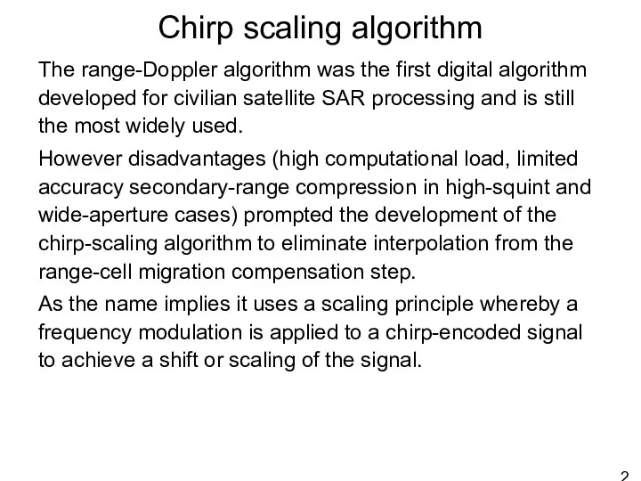
Chirp scaling algorithm
The range-Doppler algorithm was the first digital algorithm developed
Chirp scaling algorithm
The range-Doppler algorithm was the first digital algorithm developed
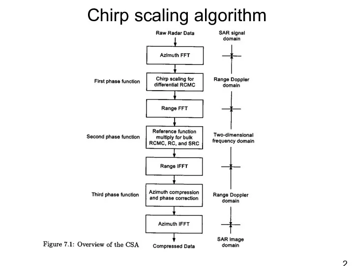
Chirp scaling algorithm
Chirp scaling algorithm
Chirp scaling algorithm
Chirp scaling algorithm
Chirp scaling algorithm
Chirp scaling algorithm
Chirp scaling algorithm
Chirp scaling algorithm
Chirp scaling algorithm
Chirp scaling algorithm
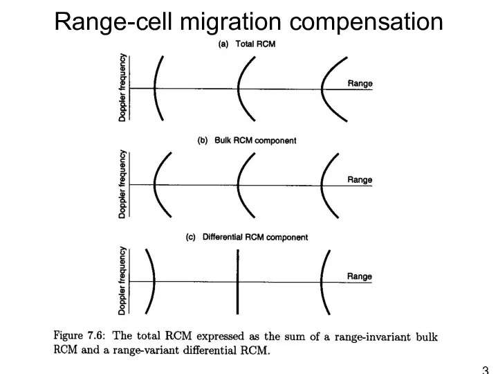
Range-cell migration compensation
Range-cell migration compensation
Omega-K algorithm (WKA)
The chirp-scaling algorithm assumes a specific form of the
Omega-K algorithm (WKA)
The chirp-scaling algorithm assumes a specific form of the
Omega-K algorithm (WKA)
Illustration of the range/azimuth cross coupling using the raw
Omega-K algorithm (WKA)
Illustration of the range/azimuth cross coupling using the raw
Omega-K algorithm (WKA)
Omega-K algorithm (WKA)
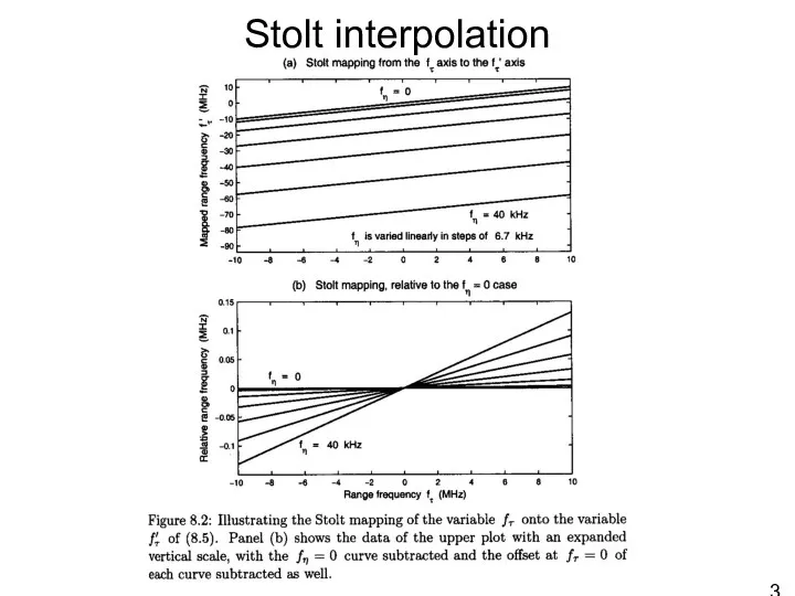
Stolt interpolation
Stolt interpolation
Stolt interpolation
Stolt interpolation
Stolt interpolation
Stolt interpolation
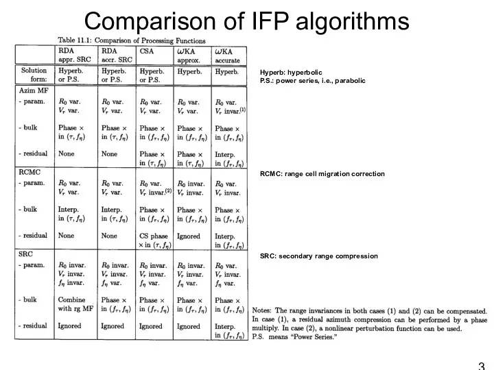
Comparison of IFP algorithms
Azim MF: azimuth matched filter
Hyperb: hyperbolic
P.S.: power series, i.e.,
Comparison of IFP algorithms
Azim MF: azimuth matched filter
Hyperb: hyperbolic
P.S.: power series, i.e.,
Motion compensation
Imperfect trajectories during SAR data collection will distort the data
Motion compensation
Imperfect trajectories during SAR data collection will distort the data
Motion compensation
To provide position and attitude knowledge various instruments are used
Gyroscopes
Motion compensation
To provide position and attitude knowledge various instruments are used
Gyroscopes
Motion compensation
Motion compensation
Motion compensation
In addition to position and attitude knowledge acquired from various
Motion compensation
In addition to position and attitude knowledge acquired from various
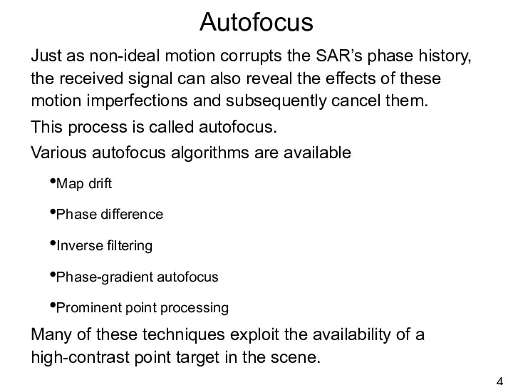
Autofocus
Just as non-ideal motion corrupts the SAR’s phase history, the received
Autofocus
Just as non-ideal motion corrupts the SAR’s phase history, the received
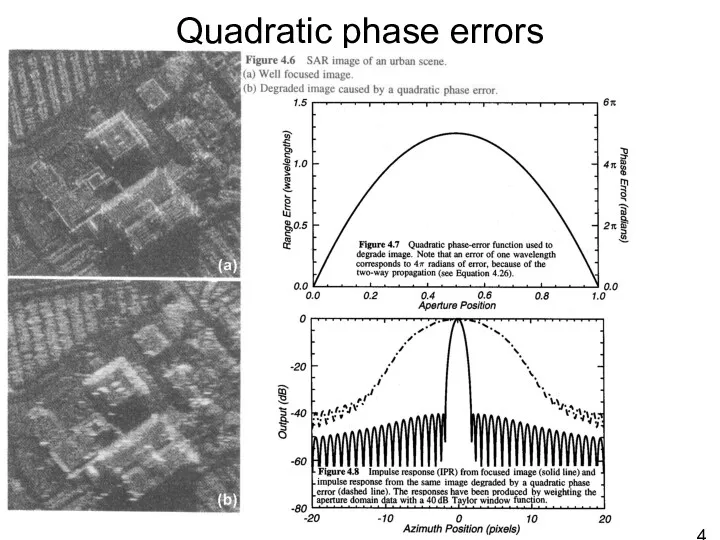
Quadratic phase errors
Quadratic phase errors
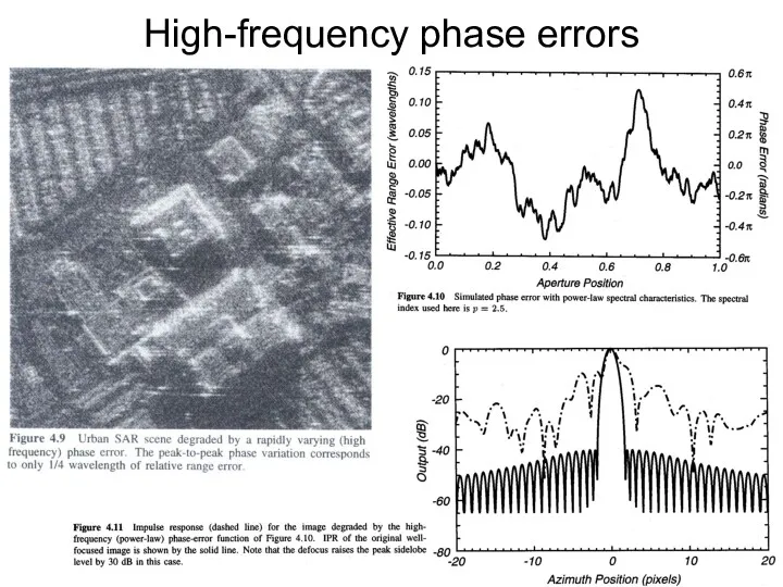
High-frequency phase errors
High-frequency phase errors
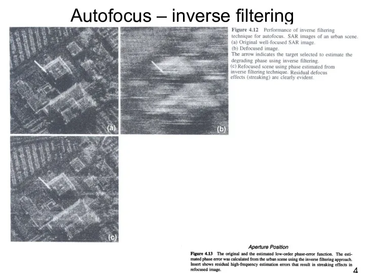
Autofocus – inverse filtering
Autofocus – inverse filtering
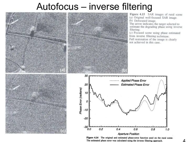
Autofocus – inverse filtering
Autofocus – inverse filtering
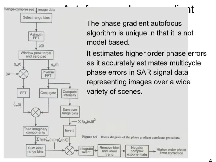
Autofocus – phase gradient
The phase gradient autofocus algorithm is unique in
Autofocus – phase gradient
The phase gradient autofocus algorithm is unique in
 Вільне падіння. Прискорення вільного падіння
 Классификация систем автоматического регулирования
 Снятие, замена приводного ремня ГРМ Chevrolet Lacetti
 Молекулярно-кинетические свойства коллоидных систем
 Презентация-игра, 7-8 класс
 Элементарные частицы
 История появления квадрокоптеров
 Делимость электрического заряда
 Урок по теме Электризация тел 8 класс
 Радиоактивность. Урок физики 9 класс
 Сила тока. Единицы силы тока
 Газораспределительный механизм
 Спидометр
 Kernfusion in der sonne
 Глава 5. Пьезоэлектрический эффект и электрострикция
 Агрегатные состояния вещества. Урок в 7 классе
 Презентация Способы изменения внутренней энергии 8 класс
 Элементы теории атомного ядра
 Шпонды және шлицты қосылыстар
 методическая разработка раздела курса физики 7 класса Давление
 Урок по теме Расчёт пути и времени движения 7 класс
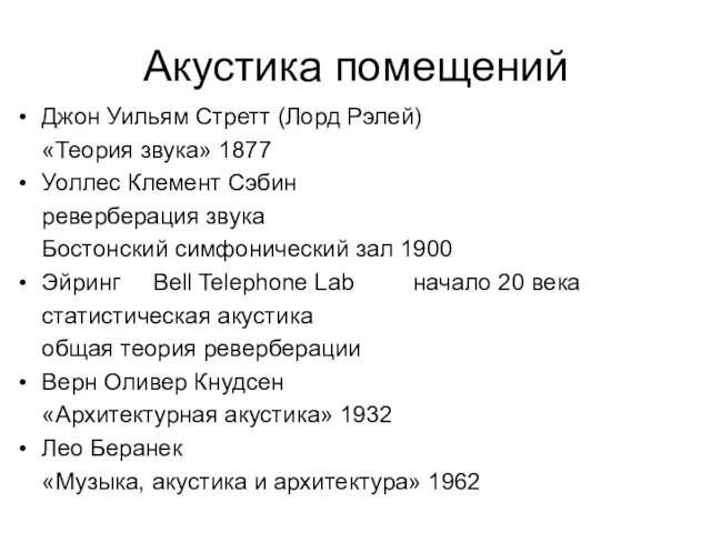 Акустика помещений
 Закон всемирного тяготения. Сила тяжести. Невесомость
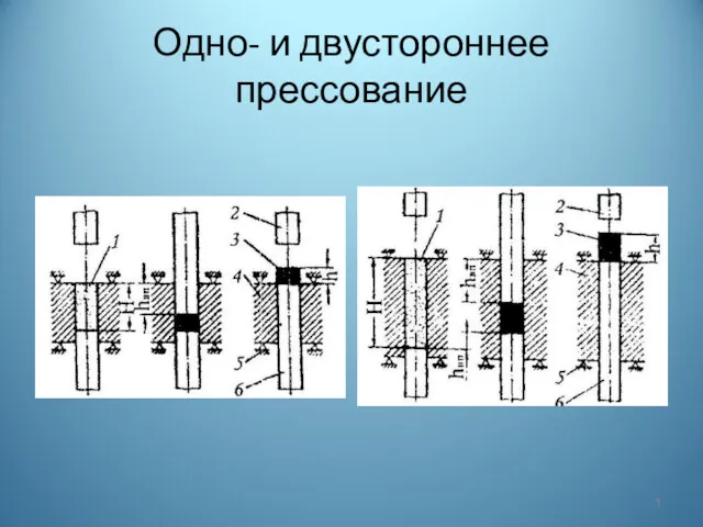 Одно- и двустороннее прессование деталей
 Количество теплоты. Единицы количества теплоты. Удельная теплоемкость. 8 класс
 сказка физического содержания Добро и зло
 Понятие о трехфазных цепях
 Основы генерирования и формирования сигналов. Лекция 2