- Dynamic Programming. Lec 10

Содержание
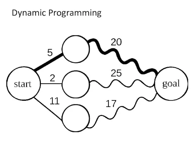
- 2. Dynamic Programming
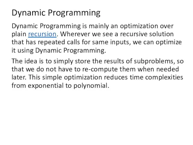
- 3. Dynamic Programming Dynamic Programming is mainly an optimization over plain recursion. Wherever we see a recursive
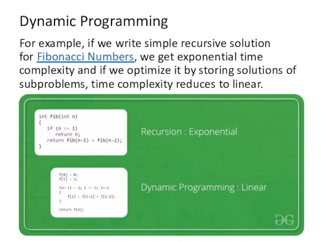
- 4. Dynamic Programming For example, if we write simple recursive solution for Fibonacci Numbers, we get exponential
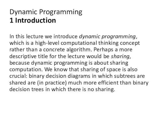
- 5. Dynamic Programming 1 Introduction In this lecture we introduce dynamic programming, which is a high-level computational
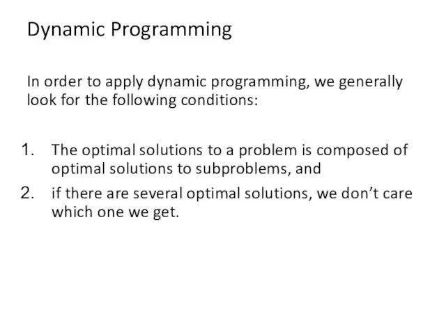
- 6. Dynamic Programming In order to apply dynamic programming, we generally look for the following conditions: The
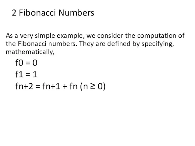
- 7. 2 Fibonacci Numbers As a very simple example, we consider the computation of the Fibonacci numbers.
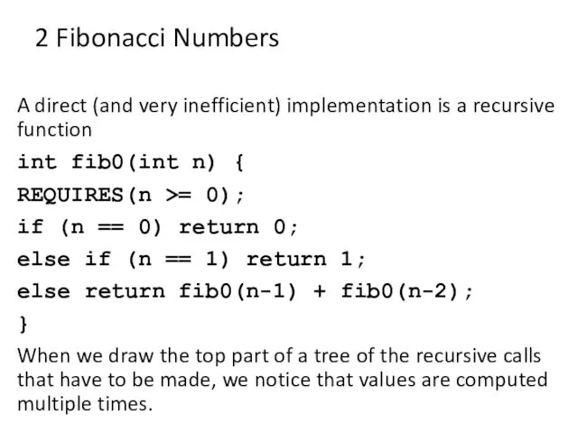
- 8. 2 Fibonacci Numbers A direct (and very inefficient) implementation is a recursive function int fib0(int n)
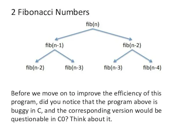
- 9. 2 Fibonacci Numbers Before we move on to improve the efficiency of this program, did you
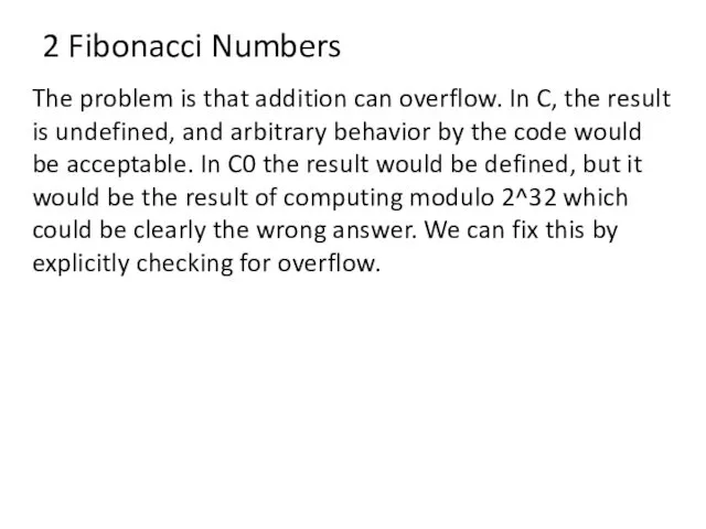
- 10. 2 Fibonacci Numbers The problem is that addition can overflow. In C, the result is undefined,
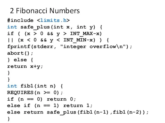
- 11. 2 Fibonacci Numbers #include int safe_plus(int x, int y) { if ( (x > 0 &&
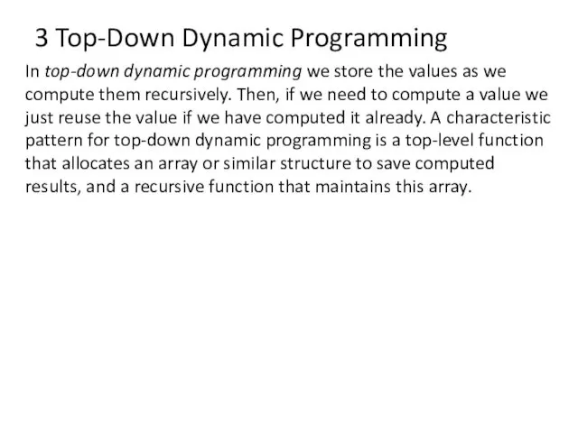
- 12. 3 Top-Down Dynamic Programming In top-down dynamic programming we store the values as we compute them
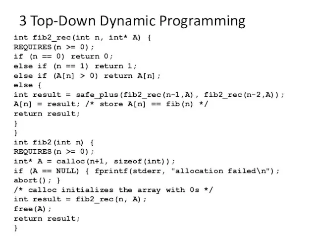
- 13. 3 Top-Down Dynamic Programming int fib2_rec(int n, int* A) { REQUIRES(n >= 0); if (n ==
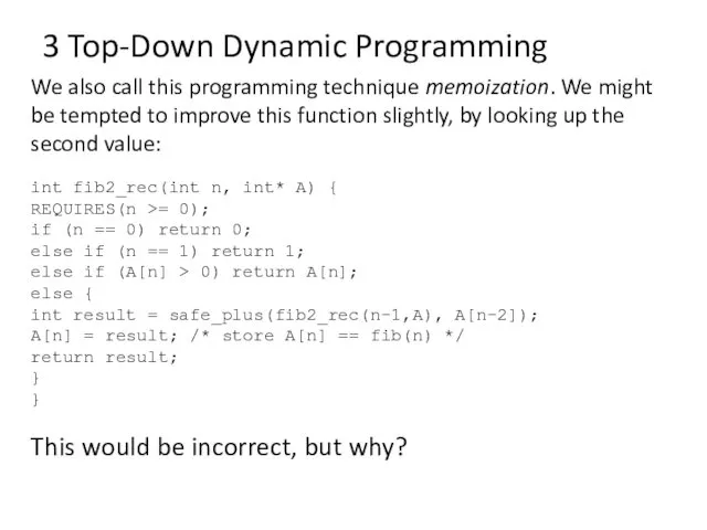
- 14. 3 Top-Down Dynamic Programming We also call this programming technique memoization. We might be tempted to
- 15. 4 Bottom-Up Dynamic Programming Top-down dynamic programming retains the structure of the original (inefficient) recursive function.
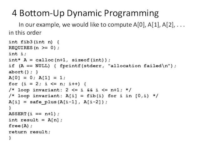
- 16. 4 Bottom-Up Dynamic Programming In our example, we would like to compute A[0], A[1], A[2], .
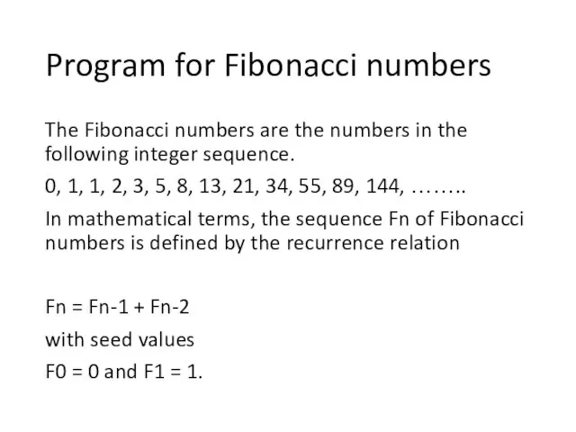
- 17. Program for Fibonacci numbers The Fibonacci numbers are the numbers in the following integer sequence. 0,
- 18. Method 1 ( Use recursion ) vs Method 2 ( Use Dynamic Programming ) Time Complexity:
- 19. Method 2 ( Use Dynamic Programming )
- 20. Method 3 ( Space Optimized Method 2 ) Time Complexity: linear O(n) Extra Space: O(1)
- 21. Method 4 ( Using power of the matrix {{1,1},{1,0}} ) This another O(n) which relies on
- 22. Method 4 ( Using power of the matrix {{1,1},{1,0}} ) #include /* Helper function that multiplies
- 23. Method 4 ( Using power of the matrix {{1,1},{1,0}} ) void multiply(int F[2][2], int M[2][2]) {
- 24. Method 4 ( Using power of the matrix {{1,1},{1,0}} ) /* Driver program to test above
- 25. Method 5 ( Optimized Method 4 ) The method 4 can be optimized to work in
- 26. Method 5 ( Optimized Method 4 ) void multiply(int F[2][2], int M[2][2]) { int x =
- 27. Method 6 (O(Log n) Time) Below is one more interesting recurrence formula that can be used
- 28. Method 6 (O(Log n) Time) Time complexity of this solution is O(Log n)
- 29. Method 7 Another approach:(Using formula) In this method we directly implement the formula for nth term
- 30. 5 BDD & ROBDD In computer science, a binary decision diagram (BDD) or branching program is
- 31. 5 Implementing ROBDDs In the implementation of ROBDDs, dynamic programming plays a pervasive role. Binary decision
- 32. 6 Encoding the n-Queens Problem The n-queens problem is to fill an n ∗ n chessboard
- 33. 6 Encoding the n-Queens Problem We would like to encode n-queens problems as ROBDDS. The idea
- 34. 6 Encoding the n-Queens Problem For example, to encode that the column 0 has at least
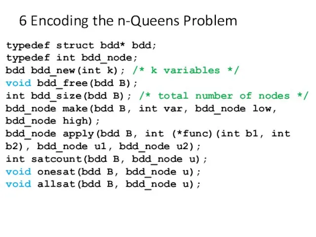
- 35. 6 Encoding the n-Queens Problem typedef struct bdd* bdd; typedef int bdd_node; bdd bdd_new(int k); /*
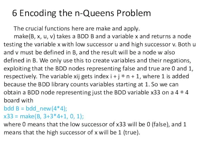
- 36. 6 Encoding the n-Queens Problem The crucial functions here are make and apply. make(B, x, u,
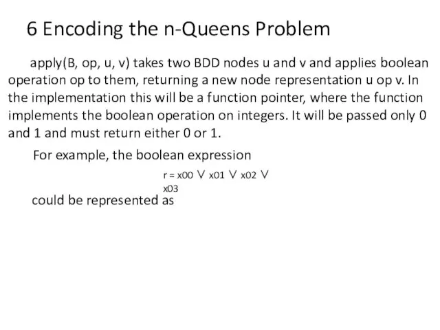
- 37. 6 Encoding the n-Queens Problem apply(B, op, u, v) takes two BDD nodes u and v
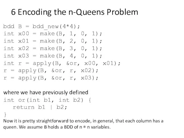
- 38. 6 Encoding the n-Queens Problem bdd B = bdd_new(4*4); int x00 = make(B, 1, 0, 1);
- 40. Скачать презентацию
Dynamic Programming
Dynamic Programming
Dynamic Programming
Dynamic Programming is mainly an optimization over plain recursion. Wherever we
Dynamic Programming
Dynamic Programming is mainly an optimization over plain recursion. Wherever we
Dynamic Programming
For example, if we write simple recursive solution for Fibonacci Numbers,
Dynamic Programming
For example, if we write simple recursive solution for Fibonacci Numbers,
Dynamic Programming
1 Introduction
In this lecture we introduce dynamic programming, which is
Dynamic Programming
1 Introduction
In this lecture we introduce dynamic programming, which is
Dynamic Programming
In order to apply dynamic programming, we generally look for
Dynamic Programming
In order to apply dynamic programming, we generally look for
2 Fibonacci Numbers
As a very simple example, we consider the
2 Fibonacci Numbers
As a very simple example, we consider the
2 Fibonacci Numbers
A direct (and very inefficient) implementation is a
2 Fibonacci Numbers
A direct (and very inefficient) implementation is a
2 Fibonacci Numbers
Before we move on to improve the efficiency
2 Fibonacci Numbers
Before we move on to improve the efficiency
2 Fibonacci Numbers
The problem is that addition can overflow. In
2 Fibonacci Numbers
The problem is that addition can overflow. In
2 Fibonacci Numbers
#include
int safe_plus(int x, int y) {
if (
2 Fibonacci Numbers
#include
int safe_plus(int x, int y) {
if (
3 Top-Down Dynamic Programming
In top-down dynamic programming we store the values
3 Top-Down Dynamic Programming
In top-down dynamic programming we store the values
3 Top-Down Dynamic Programming
int fib2_rec(int n, int* A) {
REQUIRES(n >= 0);
if
3 Top-Down Dynamic Programming
int fib2_rec(int n, int* A) {
REQUIRES(n >= 0);
if
3 Top-Down Dynamic Programming
We also call this programming technique memoization. We
3 Top-Down Dynamic Programming
We also call this programming technique memoization. We
4 Bottom-Up Dynamic Programming
Top-down dynamic programming retains the structure of the
4 Bottom-Up Dynamic Programming
Top-down dynamic programming retains the structure of the
4 Bottom-Up Dynamic Programming
In our example, we would like to compute
4 Bottom-Up Dynamic Programming
In our example, we would like to compute
Program for Fibonacci numbers
The Fibonacci numbers are the numbers in the
Program for Fibonacci numbers
The Fibonacci numbers are the numbers in the
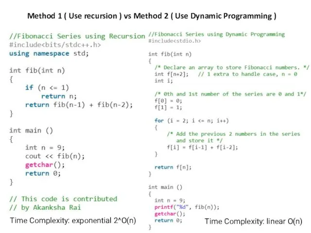
Method 1 ( Use recursion ) vs Method 2 ( Use
Method 1 ( Use recursion ) vs Method 2 ( Use
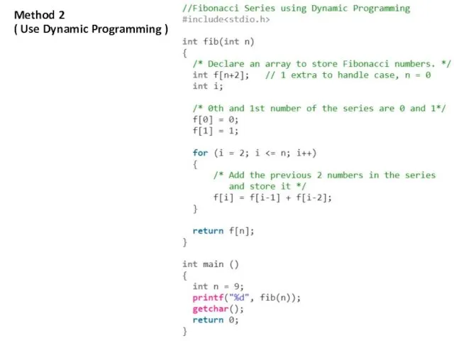
Method 2
( Use Dynamic Programming )
Method 2
( Use Dynamic Programming )
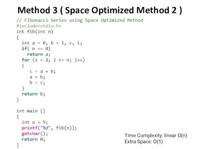
Method 3 ( Space Optimized Method 2 )
Time Complexity: linear O(n)
Extra
Method 3 ( Space Optimized Method 2 )
Time Complexity: linear O(n)
Extra
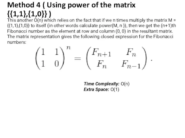
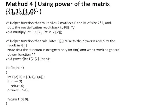
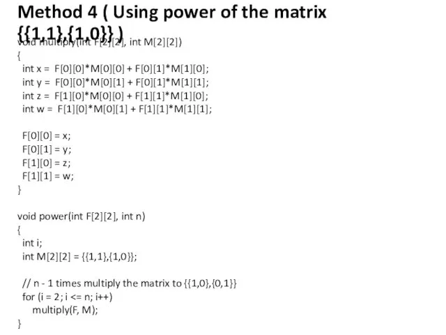
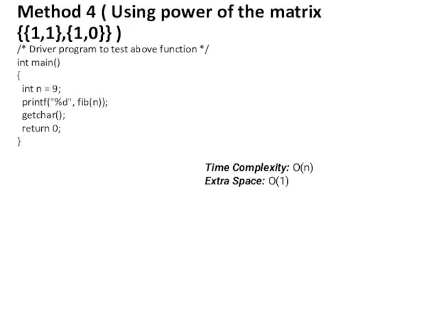
Method 4 ( Using power of the matrix {{1,1},{1,0}} )
This another
Method 4 ( Using power of the matrix {{1,1},{1,0}} )
This another
Method 4 ( Using power of the matrix {{1,1},{1,0}} )
#include
Method 4 ( Using power of the matrix {{1,1},{1,0}} )
#include
Method 4 ( Using power of the matrix {{1,1},{1,0}} )
void multiply(int
Method 4 ( Using power of the matrix {{1,1},{1,0}} )
void multiply(int
Method 4 ( Using power of the matrix {{1,1},{1,0}} )
/* Driver
Method 4 ( Using power of the matrix {{1,1},{1,0}} )
/* Driver
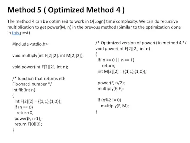
Method 5 ( Optimized Method 4 )
The method 4 can be
Method 5 ( Optimized Method 4 )
The method 4 can be
![Method 5 ( Optimized Method 4 ) void multiply(int F[2][2],](/_ipx/f_webp&q_80&fit_contain&s_1440x1080/imagesDir/jpg/21015/slide-25.jpg)
Method 5 ( Optimized Method 4 )
void multiply(int F[2][2], int M[2][2])
Method 5 ( Optimized Method 4 )
void multiply(int F[2][2], int M[2][2])
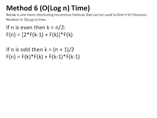
Method 6 (O(Log n) Time)
Below is one more interesting recurrence formula
Method 6 (O(Log n) Time)
Below is one more interesting recurrence formula
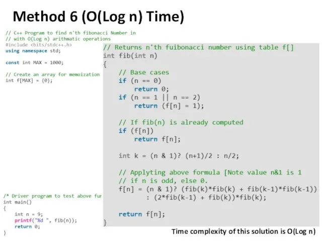
Method 6 (O(Log n) Time)
Time complexity of this solution is O(Log
Method 6 (O(Log n) Time)
Time complexity of this solution is O(Log
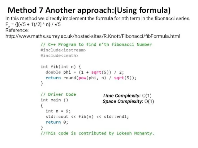
Method 7 Another approach:(Using formula)
In this method we directly implement the
Method 7 Another approach:(Using formula)
In this method we directly implement the
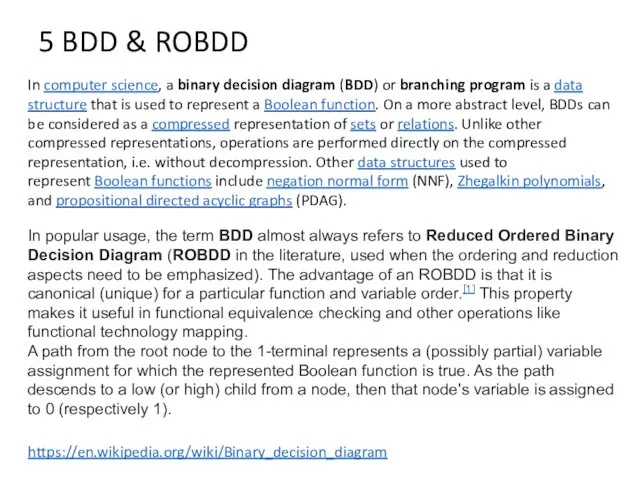
5 BDD & ROBDD
In computer science, a binary decision diagram (BDD) or branching program is a data
5 BDD & ROBDD
In computer science, a binary decision diagram (BDD) or branching program is a data
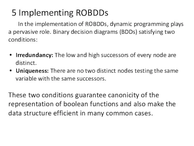
5 Implementing ROBDDs
In the implementation of ROBDDs, dynamic programming plays a
5 Implementing ROBDDs
In the implementation of ROBDDs, dynamic programming plays a
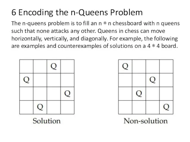
6 Encoding the n-Queens Problem
The n-queens problem is to fill an
6 Encoding the n-Queens Problem
The n-queens problem is to fill an
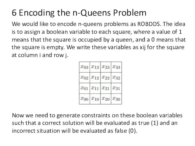
6 Encoding the n-Queens Problem
We would like to encode n-queens problems
6 Encoding the n-Queens Problem
We would like to encode n-queens problems
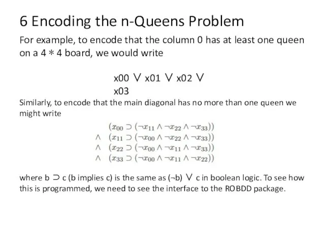
6 Encoding the n-Queens Problem
For example, to encode that the column
6 Encoding the n-Queens Problem
For example, to encode that the column
6 Encoding the n-Queens Problem
typedef struct bdd* bdd;
typedef int bdd_node;
bdd bdd_new(int
6 Encoding the n-Queens Problem
typedef struct bdd* bdd;
typedef int bdd_node;
bdd bdd_new(int
6 Encoding the n-Queens Problem
The crucial functions here are make and
6 Encoding the n-Queens Problem
The crucial functions here are make and
6 Encoding the n-Queens Problem
apply(B, op, u, v) takes two BDD
6 Encoding the n-Queens Problem
apply(B, op, u, v) takes two BDD
6 Encoding the n-Queens Problem
bdd B = bdd_new(4*4);
int x00 =
6 Encoding the n-Queens Problem
bdd B = bdd_new(4*4);
int x00 =
 Позиционные системы счисления
 Локальные сети. Параметры сетей и их стандарты
 Сбор и подготовка данных
 Современные накопители информации, используемые в вычислительной технике
 Использование технологии веб-квест как средство развития познавательных и творческих способностей учащихся
 Блочные алгоритмы. Блочное шифрование. Сравнение блочных и поточных шифров. Предпосылки создания шифра Фейстеля
 Параллельное программирование. С++. Thread Support Library. Atomic Operations Library
 Функции в Excel
 Организация и средства информационных технологий обеспечения управленческой деятельности
 Поиск публикаций и показатели деятельности ученого в Web of Science
 Бездротові мережі
 Занятие 1. Знакомство с программой Adobe Photoshop
 Microsoft Visual Studio — линейка продуктов компании Microsoft
 Операторы цикла
 Понятие об информации. Представление информации. Информационная деятельность человека.
 Автоматизоване створення запитів у базі даних
 Архітектура операційних систем
 Windows System Programming
 Личный кабинет
 Мир станочника. Аддитивные технологии и 3D-сканирование
 Методы и средства защиты программ от компьютерных вирусов
 46_Yaroslavskaya_Sasha
 Локальные и глобальные сети ЭВМ. Защита информации в сетях. (Тема 6)
 Godseeker. Игра
 Рабочий стол. Управление компьютером с помощью мыши
 Проектирование изделий из листового металла в NX
 Эти люди изменили мир
 Электронные ресурсы для детей и юношества в общедоступных библиотеках: создание и использование