- Tuning SQL query performance

Содержание
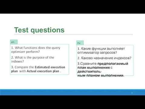
- 2. Test questions 1. What functions does the query optimizer perform? 2. What is the purpose of
- 3. Contents 1. Query Processing 2. Database Indexes 3. Query Analysis Tools 4. Query tuning practice
- 4. 1. Query Processing
- 5. 1.1. End User Interaction with DBMS End users interact with the DBMS through the use of
- 6. Query Processing includes translations on high level Queries into low level expressions that can be used
- 7. Importance: The goal of query optimization is to reduce the system resources required to fulfill a
- 8. A single query can be executed through different algorithms or re-written in different forms and structures.
- 9. Query Optimizer is often a cost-based optimizer. It assigns a number called cost to each possible
- 10. Since database structures are complex, in most cases, and especially for not-very-simple queries, the needed data
- 11. 2. Database Indexes
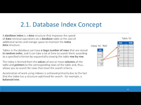
- 12. A database index is a data structure that improves the speed of data retrieval operations on
- 13. Clustered indexes sort and store the data rows in the table or view based on their
- 14. Nonclustered index contains the nonclustered index key values and each key value entry has a pointer
- 15. When you create a table with a Primary Key, SQL Server automatically creates a corresponding clustered
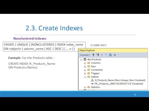
- 16. Example. For the Products table : CREATE INDEX IX_Products_Name ON Products (Name); 2.3. Create Indexes Nonclustered
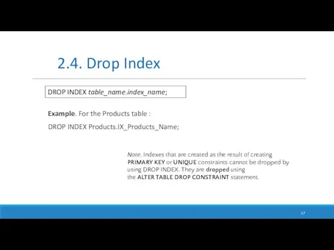
- 17. Example. For the Products table : DROP INDEX Products.IX_Products_Name; 2.4. Drop Index DROP INDEX table_name.index_name; Note.
- 18. 2.5. Looking for indexes sp_helpindex is a system stored procedure which lists the information of all
- 19. 2.5. Looking for indexes sp_helpindex is a system stored procedure which lists the information of all
- 20. 3. Query Analysis Tools
- 21. STATISTICS IO will tell you the cost of the query in terms of the actual number
- 22. Displays the number of milliseconds required to parse, compile, and execute each statement. 3.2. STATISTICS TIME
- 23. Execution plans can tell you how a query will be executed, or how a query was
- 24. In the Query Editor window, click the Display Estimated Execution Plan icon on the tool bar.
- 25. 1. In the Query Editor window, click the Include Actual Execution Plan icon on the tool
- 26. Usually, you read a graphical execution plan from right to left and top to bottom. The
- 27. Execution plans can tell you how a query will be executed, or how a query was
- 28. 3.8. Operator Descriptions https://docs.microsoft.com/en-us/sql/relational-databases/showplan-logical-and-physical-operators-reference?view=sql-server-ver15
- 29. 4. Query tuning practice
- 30. Identify relevant stakeholders. (All involved parties + DBA) Focus on business outcomes. Be sure the query
- 31. DBMS should scan column names and replace * with actual table columns. 4.2. Avoid SELECT *
- 32. DBMS should scan column names and replace * with actual table columns. 4.2. Avoid SELECT *
- 33. SELECT DISTINCT is a handy way to remove duplicates from a query. SELECT DISTINCT works by
- 34. In some databases, this type of queries are inefficient as it first creates temp data with
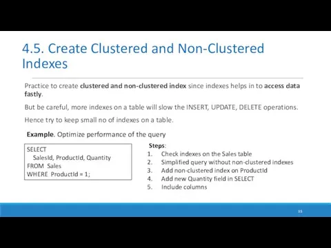
- 35. Practice to create clustered and non-clustered index since indexes helps in to access data fastly. But
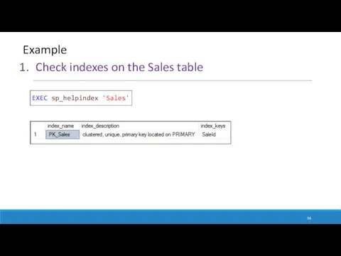
- 36. EXEC sp_helpindex 'Sales' Check indexes on the Sales table Example
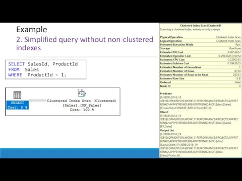
- 37. 2. Simplified query without non-clustered indexes Example SELECT SalesId, ProductId FROM Sales WHERE ProductId = 1;
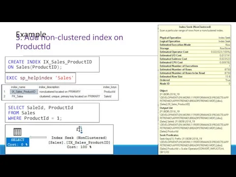
- 38. 3. Add non-clustered index on ProductId Example CREATE INDEX IX_Sales_ProductID ON Sales(ProductID); EXEC sp_helpindex 'Sales' SELECT
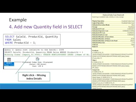
- 39. 4. Add new Quantity field in SELECT Example SELECT SaleId, ProductId, Quantity FROM Sales WHERE ProductId
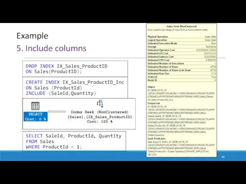
- 40. 5. Include columns Example DROP INDEX IX_Sales_ProductID ON Sales(ProductID); CREATE INDEX IX_Sales_ProductID_Inc ON Sales (ProductId) INCLUDE
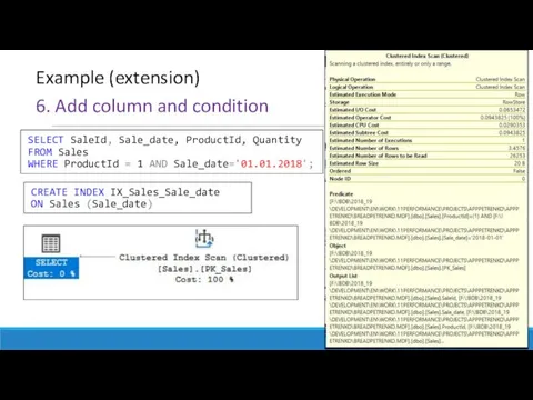
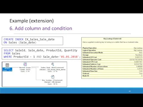
- 41. 6. Add column and condition Example (extension) CREATE INDEX IX_Sales_Sale_date ON Sales (Sale_date) SELECT SaleId, Sale_date,
- 42. 6. Add column and condition Example (extension) CREATE INDEX IX_Sales_Sale_date ON Sales (Sale_date) SELECT SaleId, Sale_date,
- 43. 6. Add column and condition Example (extension- from tips) DROP INDEX IX_Sales_Sale_date ON Sales; SELECT SaleId,
- 45. Скачать презентацию
Test questions
1. What functions does the query optimizer perform?
2. What is
Test questions
1. What functions does the query optimizer perform?
2. What is
Contents
1. Query Processing
2. Database Indexes
3. Query Analysis Tools
4. Query tuning practice
Contents
1. Query Processing
2. Database Indexes
3. Query Analysis Tools
4. Query tuning practice
1. Query Processing
1. Query Processing
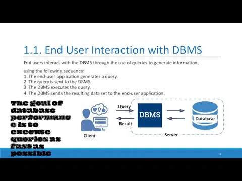
1.1. End User Interaction with DBMS
End users interact with the DBMS
1.1. End User Interaction with DBMS
End users interact with the DBMS
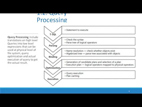
Query Processing includes translations on high level Queries into low level expressions
Query Processing includes translations on high level Queries into low level expressions
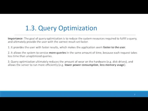
Importance: The goal of query optimization is to reduce the system
Importance: The goal of query optimization is to reduce the system
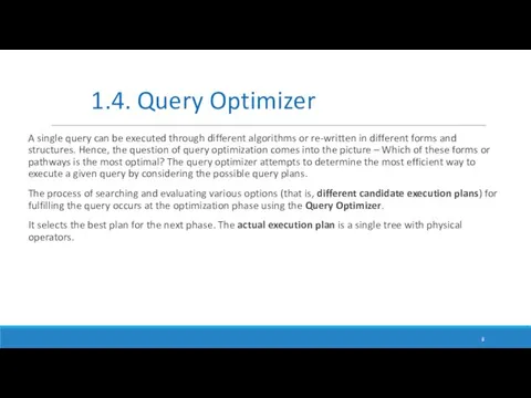
A single query can be executed through different algorithms or re-written
A single query can be executed through different algorithms or re-written
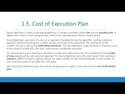
Query Optimizer is often a cost-based optimizer. It assigns a number
Query Optimizer is often a cost-based optimizer. It assigns a number
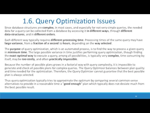
Since database structures are complex, in most cases, and especially for
Since database structures are complex, in most cases, and especially for
2. Database Indexes
2. Database Indexes
A database index is a data structure that improves the speed of data retrieval operations on a database table
A database index is a data structure that improves the speed of data retrieval operations on a database table
Clustered indexes sort and store the data rows in the table
Clustered indexes sort and store the data rows in the table
Nonclustered index contains the nonclustered index key values and each key
Nonclustered index contains the nonclustered index key values and each key
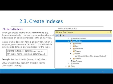
When you create a table with a Primary Key, SQL Server automatically
When you create a table with a Primary Key, SQL Server automatically
Example. For the Products table :
CREATE INDEX IX_Products_Name
ON Products (Name);
2.3.
Example. For the Products table :
CREATE INDEX IX_Products_Name
ON Products (Name);
2.3.
Example. For the Products table :
DROP INDEX Products.IX_Products_Name;
2.4. Drop Index
DROP INDEX table_name.index_name;
Note. Indexes
Example. For the Products table :
DROP INDEX Products.IX_Products_Name;
2.4. Drop Index
DROP INDEX table_name.index_name;
Note. Indexes
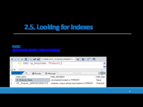
2.5. Looking for indexes
sp_helpindex is a system stored procedure which lists
2.5. Looking for indexes
sp_helpindex is a system stored procedure which lists
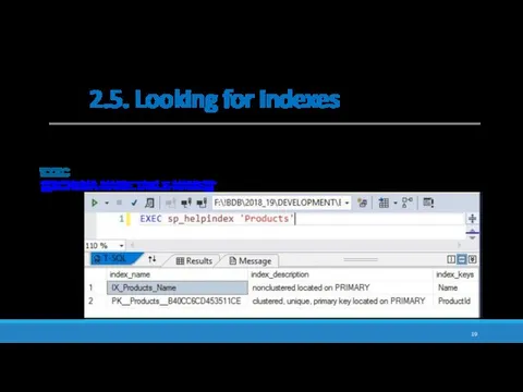
2.5. Looking for indexes
sp_helpindex is a system stored procedure which lists
2.5. Looking for indexes
sp_helpindex is a system stored procedure which lists
3. Query Analysis Tools
3. Query Analysis Tools
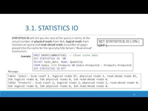
STATISTICS IO will tell you the cost of the query in
STATISTICS IO will tell you the cost of the query in
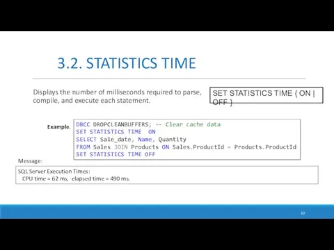
Displays the number of milliseconds required to parse, compile, and execute
Displays the number of milliseconds required to parse, compile, and execute
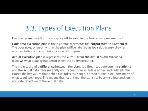
Execution plans can tell you how a query will be executed,
Execution plans can tell you how a query will be executed,
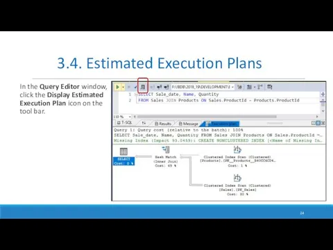
In the Query Editor window, click the Display Estimated Execution Plan
In the Query Editor window, click the Display Estimated Execution Plan
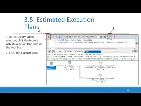
1. In the Query Editor window, click the Include Actual Execution
1. In the Query Editor window, click the Include Actual Execution
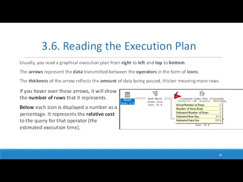
Usually, you read a graphical execution plan from right to left
Usually, you read a graphical execution plan from right to left
Execution plans can tell you how a query will be executed,
Execution plans can tell you how a query will be executed,
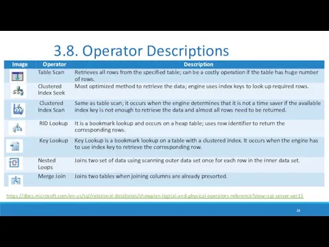
3.8. Operator Descriptions
https://docs.microsoft.com/en-us/sql/relational-databases/showplan-logical-and-physical-operators-reference?view=sql-server-ver15
3.8. Operator Descriptions
https://docs.microsoft.com/en-us/sql/relational-databases/showplan-logical-and-physical-operators-reference?view=sql-server-ver15
4. Query tuning practice
4. Query tuning practice
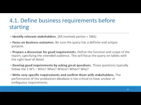
Identify relevant stakeholders. (All involved parties + DBA)
Focus on
Identify relevant stakeholders. (All involved parties + DBA)
Focus on

DBMS should scan column names and replace * with actual table
DBMS should scan column names and replace * with actual table
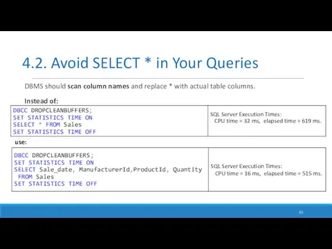
DBMS should scan column names and replace * with actual table
DBMS should scan column names and replace * with actual table
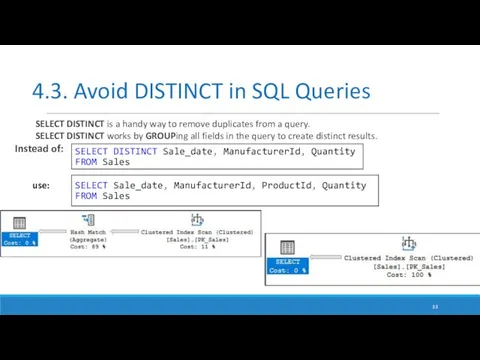
SELECT DISTINCT is a handy way to remove duplicates from a query.
SELECT
SELECT DISTINCT is a handy way to remove duplicates from a query.
SELECT
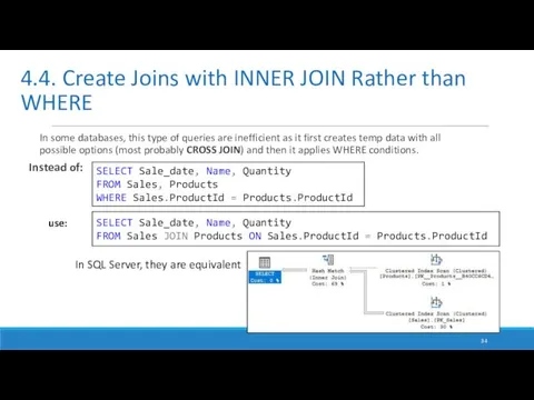
In some databases, this type of queries are inefficient as it
In some databases, this type of queries are inefficient as it
Practice to create clustered and non-clustered index since indexes helps in
Practice to create clustered and non-clustered index since indexes helps in
EXEC sp_helpindex 'Sales'
Check indexes on the Sales table
Example
EXEC sp_helpindex 'Sales'
Check indexes on the Sales table
Example
2. Simplified query without non-clustered indexes
Example
SELECT SalesId, ProductId
FROM Sales
WHERE ProductId =
2. Simplified query without non-clustered indexes
Example
SELECT SalesId, ProductId
FROM Sales
WHERE ProductId =
3. Add non-clustered index on ProductId
Example
CREATE INDEX IX_Sales_ProductID
ON Sales(ProductID);
EXEC sp_helpindex
3. Add non-clustered index on ProductId
Example
CREATE INDEX IX_Sales_ProductID
ON Sales(ProductID);
EXEC sp_helpindex
4. Add new Quantity field in SELECT
Example
SELECT SaleId, ProductId, Quantity
FROM
4. Add new Quantity field in SELECT
Example
SELECT SaleId, ProductId, Quantity
FROM
5. Include columns
Example
DROP INDEX IX_Sales_ProductID
ON Sales(ProductID);
CREATE INDEX IX_Sales_ProductID_Inc
ON Sales (ProductId)
INCLUDE
5. Include columns
Example
DROP INDEX IX_Sales_ProductID
ON Sales(ProductID);
CREATE INDEX IX_Sales_ProductID_Inc
ON Sales (ProductId)
INCLUDE
6. Add column and condition
Example (extension)
CREATE INDEX IX_Sales_Sale_date
ON Sales (Sale_date)
SELECT SaleId,
6. Add column and condition
Example (extension)
CREATE INDEX IX_Sales_Sale_date
ON Sales (Sale_date)
SELECT SaleId,
6. Add column and condition
Example (extension)
CREATE INDEX IX_Sales_Sale_date
ON Sales (Sale_date)
SELECT SaleId,
6. Add column and condition
Example (extension)
CREATE INDEX IX_Sales_Sale_date
ON Sales (Sale_date)
SELECT SaleId,
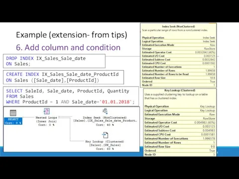
6. Add column and condition
Example (extension- from tips)
DROP INDEX IX_Sales_Sale_date
ON
6. Add column and condition
Example (extension- from tips)
DROP INDEX IX_Sales_Sale_date
ON
 Интеллектуальная игра Хакеры
 Использование современных наукометрических показателей
 Memory management. Implementation issues & segmentation
 Управление информационной безопасности в НРД. Первичный инструктаж
 Использование элементов алгебры логики при решении заданий ЕГЭ по информатике
 Технические и программные средства реализации информационных процессов. Обзор офисных приложений
 Как найти себя в ИТ. Существующие направления в ИТ
 1С:ERP. Управление предприятием
 Scheduling. Introduction
 Пошук інформації в інтернеті
 Программное обеспечение компьютера
 Разветвляющиеся алгоритмы на языке Паскаль
 Системы для математической обработки данных
 Компьютерная презентация к уроку 4 по теме Интернет-зависимость.
 Архитектура компьютеров. Общие принципы работы компьютеров
 Operating system. Applications
 Конспект интегрированного урока ИЗО и информатики
 Типы данных
 Алгоритмическая конструкция ветвление
 Human-computer interaction
 Формирование запросов в базах данных
 Статические модели объектно-ориентированных ИС. Лекция 3
 Знакомство с TrikStudio
 Бақылаудың функциялары және түрлері
 Информационные технологии на автомобильном транспорте
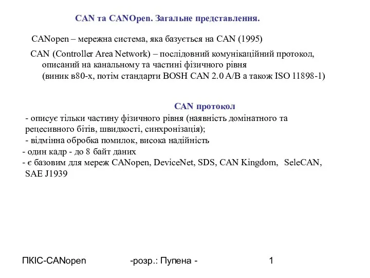 CAN та CANOpen. Загальне представлення
 Оценка количества информации
 Технологии компьютерной анимации