- D2D wireless connection modeling for moving devices in 5G technology

Содержание
- 2. The problem in general
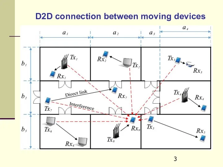
- 3. D2D connection between moving devices
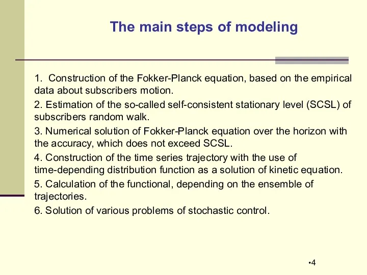
- 4. The main steps of modeling 1. Construction of the Fokker-Planck equation, based on the empirical data
- 5. Generation of non-stationary trajectories of random walk
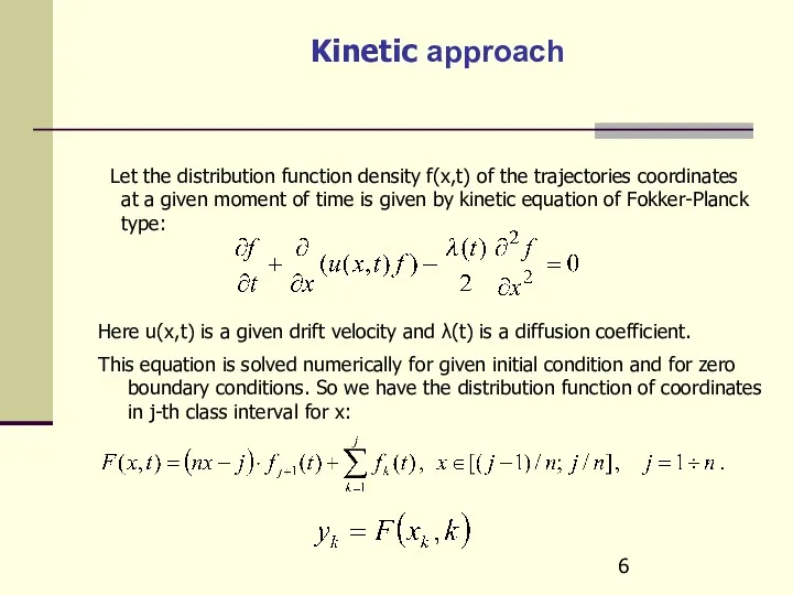
- 6. Kinetic approach Let the distribution function density f(x,t) of the trajectories coordinates at a given moment
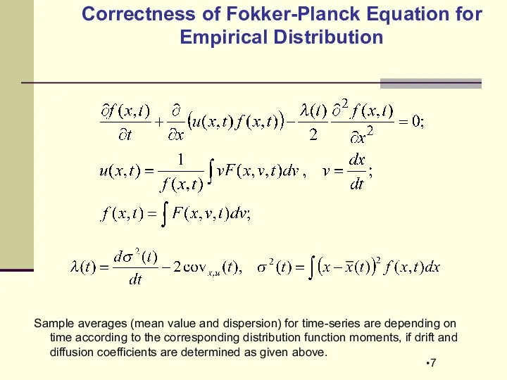
- 7. Correctness of Fokker-Planck Equation for Empirical Distribution Sample averages (mean value and dispersion) for time-series are
- 8. Explicit scheme for t with right pattern for the second derivative over x is unstable: So
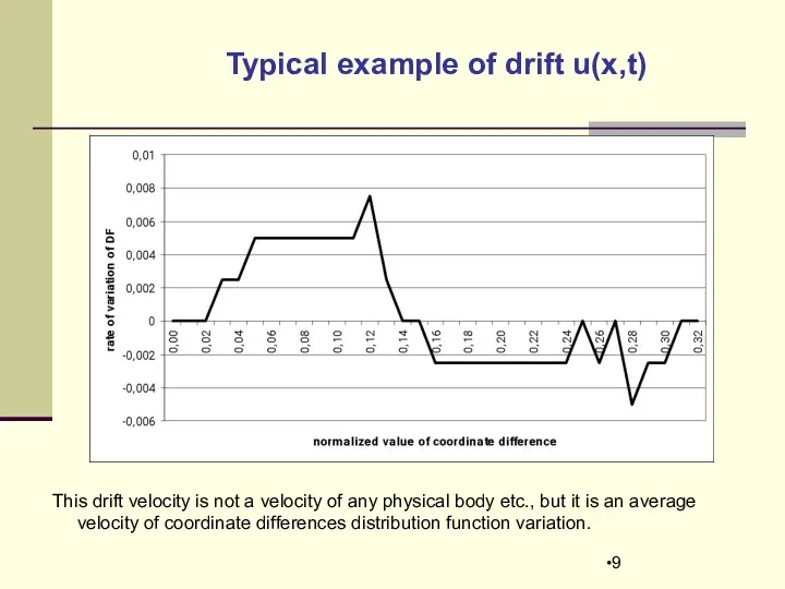
- 9. Typical example of drift u(x,t) This drift velocity is not a velocity of any physical body
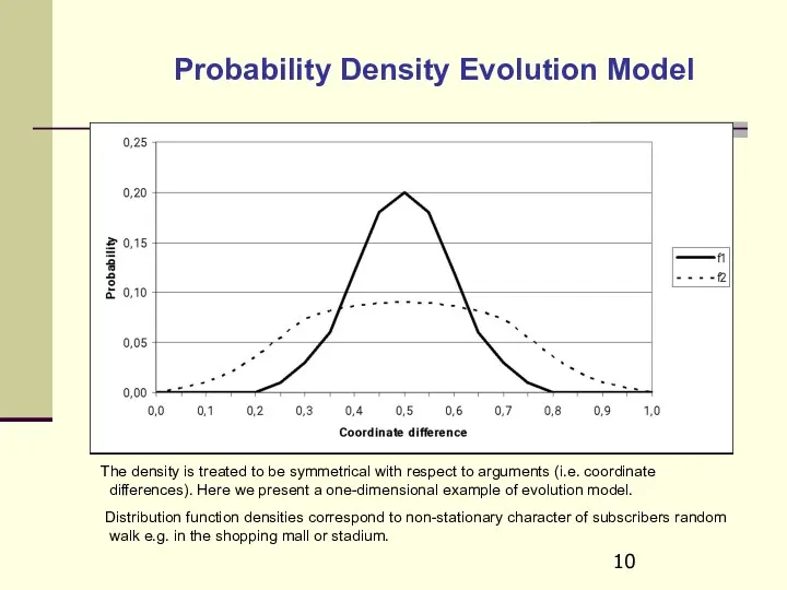
- 10. Probability Density Evolution Model The density is treated to be symmetrical with respect to arguments (i.e.
- 11. Example of trajectories ensemble simulation
- 12. For any given set volume N we construct the distribution function G of distances between distribution
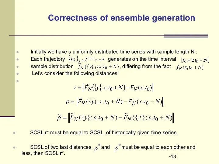
- 13. Correctness of ensemble generation Initially we have s uniformly distributed time series with sample length N
- 14. SIR Indicator Trajectory
- 15. SIR value in a continuous media From the previous step we have N random trajectories i=1,2,…,N
- 16. Example of 10 trajectories in square with reflection boundary conditions
- 17. Let us derive the evolution equation for average SIR value where f(r,t) is satisfied to the
- 18. Final Evolution Equation for Average SIR
- 19. SIR dispersion evolution equation – 1 Let us consider a SIR variance Then we obtain And
- 20. SIR dispersion evolution equation – 2 So we see, that it is very complex non-linear with
- 21. Stability D2D connection indicator If q(t)>1, the connection can be treated as a stable one, even
- 22. SIR Indicator Distribution Function
- 23. Typical SIR trajectory and SIR distribution
- 24. SIR DFD vs diffusion for zero drift
- 25. SIR DFD vs drift for zero diffusion
- 26. Analysis of D2D connection stability
- 27. The SIR standard deviation We consider two cases, i.e. two ensembles of trajectories: s(t) 1 (for
- 28. Indicator of stability We consider two cases, i.e. two ensembles of trajectories: s(t) 1 (for this
- 29. The SIR Simulation The first case (q>1) is more stable, than the second one (q
- 30. Distribution Function of the first break down moment
- 31. Simulation of empirical distribution function of the first break down moment Distribution functions of the first
- 32. Classical result for Brownian motion If the SIR behavior can be approximated by a standard Wiener
- 33. Simulation DFD for non-stationary random walk of subscribers The asymptotical bechaviour of DFD for large time
- 34. Analysis of cashing effects
- 35. Simulation results for DFD first break down with cashing T=1 T=2 On the horizontal axe –
- 36. Empirical dependence of the maximum continuity period on the cashing value
- 37. The type of normalized DFD
- 38. Conclusions Numerical simulation the SIR trajectory for an arbitrary pare of abonents, based on the random
- 39. The main references 1. Orlov Yu.N., Fedorov S.L. 2016. Modelirovanie raspredelenij funkcionalov na ansamble traektorij nestatsionarnogo
- 41. Скачать презентацию
The problem in general
The problem in general
D2D connection between moving devices
D2D connection between moving devices
The main steps of modeling
1. Construction of the Fokker-Planck equation, based
The main steps of modeling
1. Construction of the Fokker-Planck equation, based
Generation
of non-stationary trajectories
of random walk
Generation
of non-stationary trajectories
of random walk
Kinetic approach
Let the distribution function density f(x,t) of the trajectories
Kinetic approach
Let the distribution function density f(x,t) of the trajectories
Correctness of Fokker-Planck Equation for Empirical Distribution
Sample averages (mean value
Correctness of Fokker-Planck Equation for Empirical Distribution
Sample averages (mean value
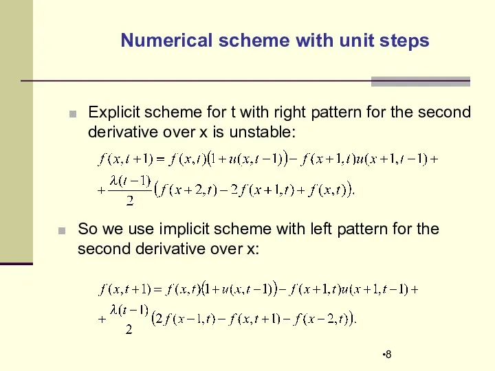
Explicit scheme for t with right pattern for the second derivative
Explicit scheme for t with right pattern for the second derivative
Typical example of drift u(x,t)
This drift velocity is not
Typical example of drift u(x,t)
This drift velocity is not
Probability Density Evolution Model
The density is treated to be symmetrical
Probability Density Evolution Model
The density is treated to be symmetrical
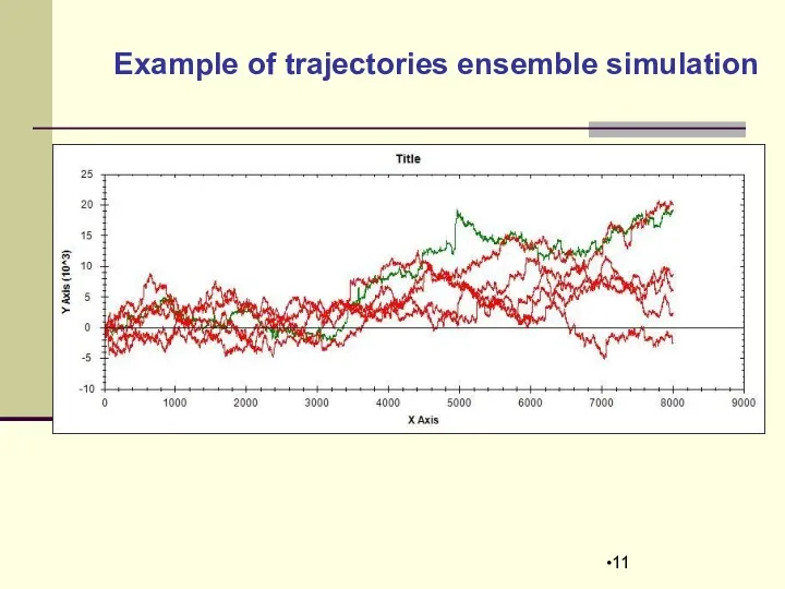
Example of trajectories ensemble simulation
Example of trajectories ensemble simulation
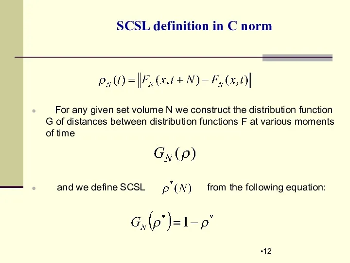
For any given set volume N we construct the distribution
For any given set volume N we construct the distribution
Correctness of ensemble generation
Initially we have s uniformly distributed time
Correctness of ensemble generation
Initially we have s uniformly distributed time
SIR Indicator
Trajectory
SIR Indicator
Trajectory
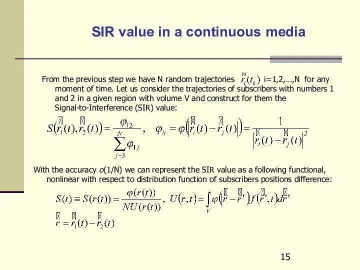
SIR value in a continuous media
From the previous step we have
SIR value in a continuous media
From the previous step we have
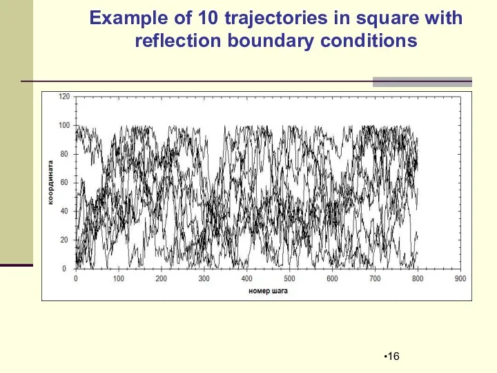
Example of 10 trajectories in square with reflection boundary conditions
Example of 10 trajectories in square with reflection boundary conditions
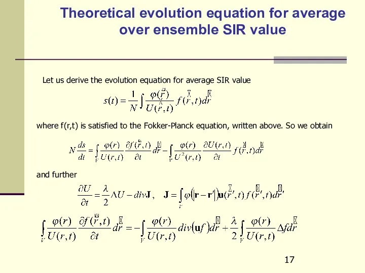
Let us derive the evolution equation for average SIR value
where f(r,t)
Let us derive the evolution equation for average SIR value
where f(r,t)
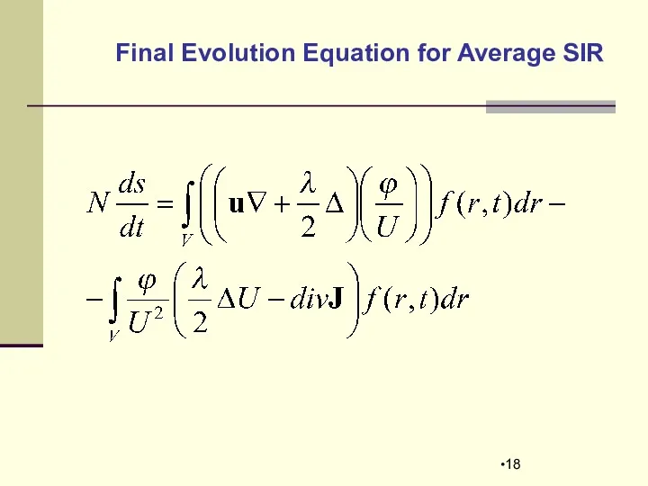
Final Evolution Equation for Average SIR
Final Evolution Equation for Average SIR
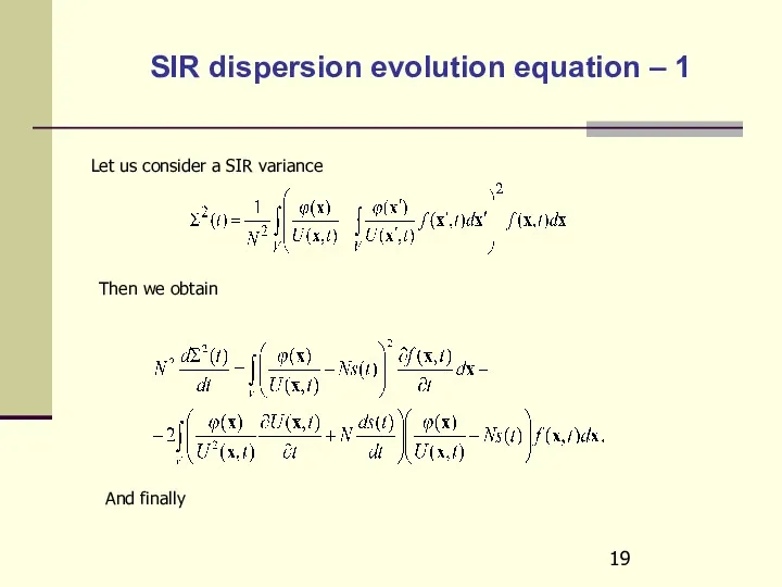
SIR dispersion evolution equation – 1
Let us consider a SIR
SIR dispersion evolution equation – 1
Let us consider a SIR
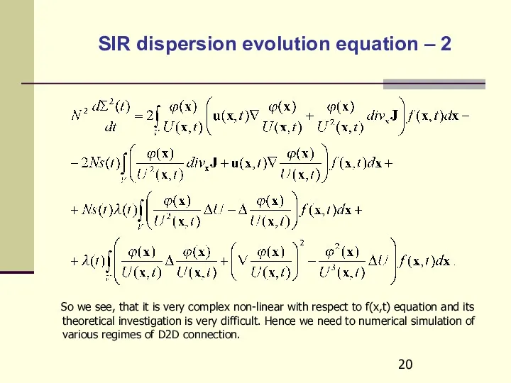
SIR dispersion evolution equation – 2
So we see, that
SIR dispersion evolution equation – 2
So we see, that
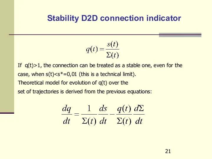
Stability D2D connection indicator
If q(t)>1, the connection can be treated
Stability D2D connection indicator
If q(t)>1, the connection can be treated
SIR Indicator
Distribution Function
SIR Indicator
Distribution Function
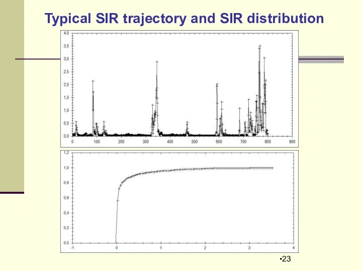
Typical SIR trajectory and SIR distribution
Typical SIR trajectory and SIR distribution
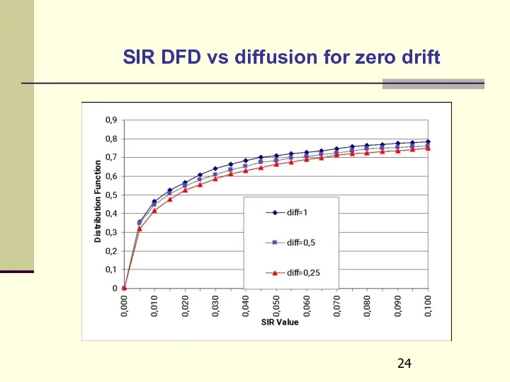
SIR DFD vs diffusion for zero drift
SIR DFD vs diffusion for zero drift
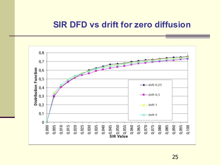
SIR DFD vs drift for zero diffusion
SIR DFD vs drift for zero diffusion
Analysis of D2D
connection stability
Analysis of D2D
connection stability
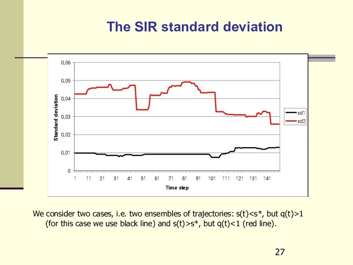
The SIR standard deviation
We consider two cases, i.e. two ensembles
The SIR standard deviation
We consider two cases, i.e. two ensembles
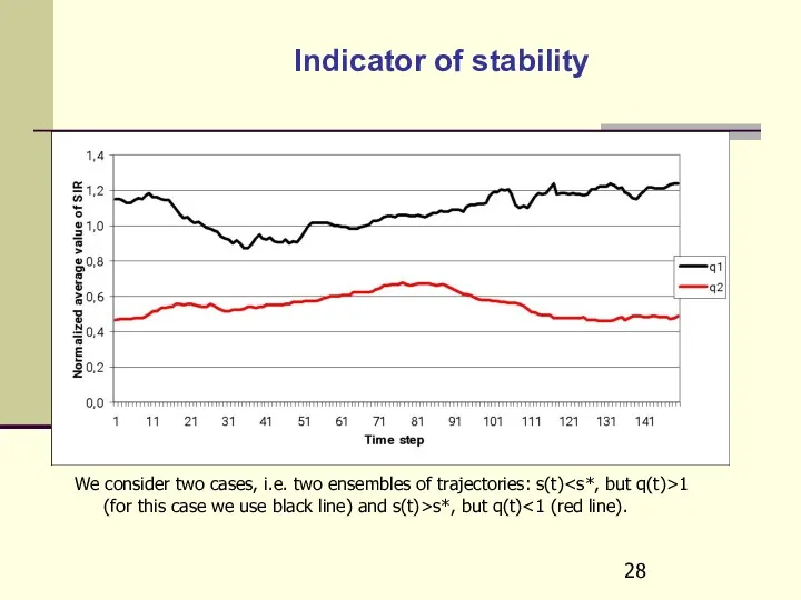
Indicator of stability
We consider two cases, i.e. two ensembles of
Indicator of stability
We consider two cases, i.e. two ensembles of
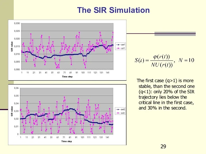
The SIR Simulation
The first case (q>1) is more stable,
The SIR Simulation
The first case (q>1) is more stable,
Distribution Function
of the first break down moment
Distribution Function
of the first break down moment
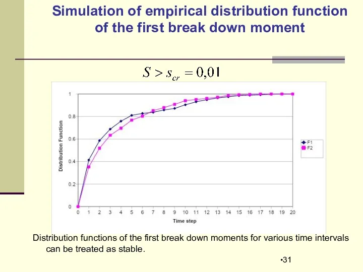
Simulation of empirical distribution function of the first break down moment
Simulation of empirical distribution function of the first break down moment
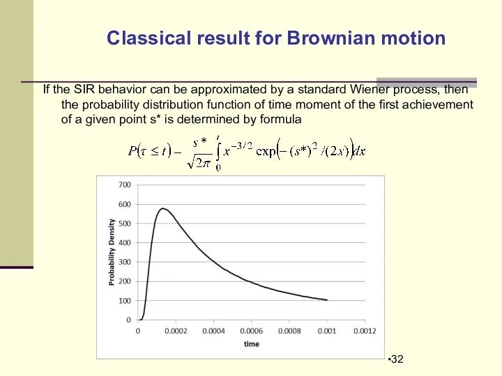
Classical result for Brownian motion
If the SIR behavior can be
Classical result for Brownian motion
If the SIR behavior can be
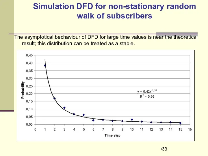
Simulation DFD for non-stationary random walk of subscribers
The asymptotical bechaviour
Simulation DFD for non-stationary random walk of subscribers
The asymptotical bechaviour
Analysis of cashing effects
Analysis of cashing effects
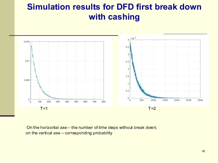
Simulation results for DFD first break down with cashing
T=1
T=2
Simulation results for DFD first break down with cashing
T=1
T=2
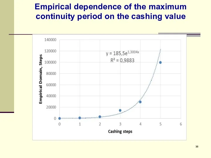
Empirical dependence of the maximum continuity period on the cashing value
Empirical dependence of the maximum continuity period on the cashing value
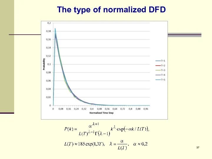
The type of normalized DFD
The type of normalized DFD
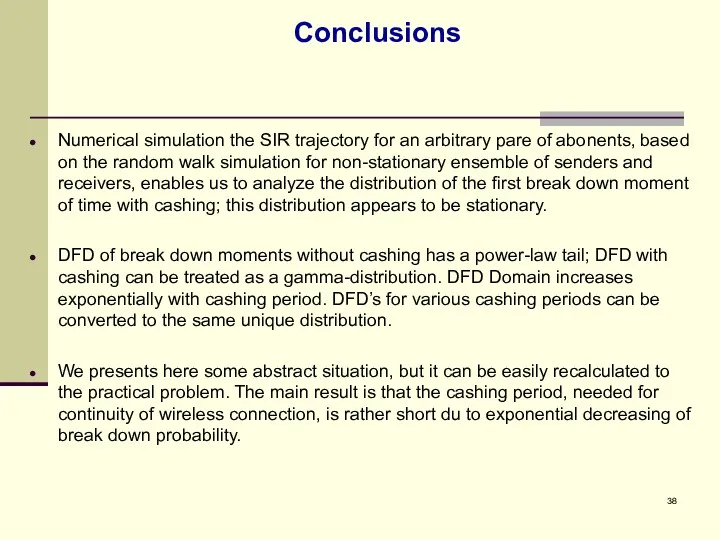
Conclusions
Numerical simulation the SIR trajectory for an arbitrary pare of abonents,
Conclusions
Numerical simulation the SIR trajectory for an arbitrary pare of abonents,

The main references
1. Orlov Yu.N., Fedorov S.L. 2016. Modelirovanie raspredelenij funkcionalov
The main references
1. Orlov Yu.N., Fedorov S.L. 2016. Modelirovanie raspredelenij funkcionalov
 Формула Пика
 Практикум по решению ключевых задач по теории вероятностей (ЕГЭ). 11 класс
 Площади фигур
 Математические методы в психологии
 Движение вдогонку
 Разложение многочленов на множители. Готовимся к ГИА!
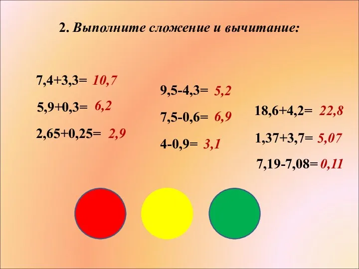 Сложение и вычитание десятичных дробей
 Решение уравнения cosx = a. Понятие арккосинуса числа
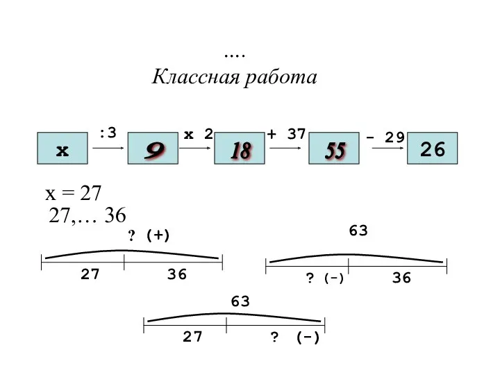 Урок математики во 2 классе по теме: Уравнения.
 Краски радуги Диск
 20181128_umnozhenie_mnogochlena_na_mnogochlen
 Тренажер по теме Больше, меньше, либо равно. 1 класс
 Логарифмы на ЕГЭ
 Сложение и вычитание векторов
 Неравенства
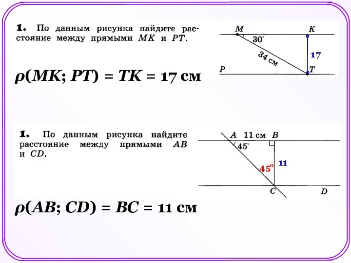 Построение треугольника по трём элементам
 Умножение разности двух выражений на их сумму
 Сложение числа 2 с однозначными числами 1 класс
 Решение дробно-рациональных уравнений с параметром
 С новым годом, второклашки!
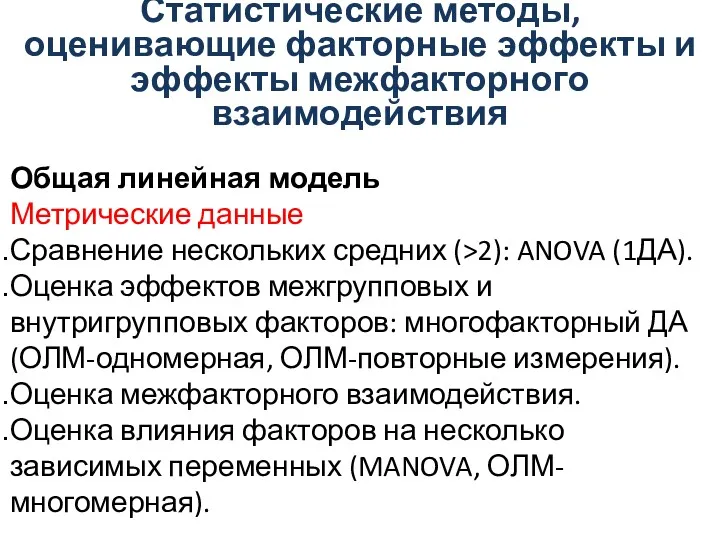 Статистические методы, оценивающие факторные эффекты и эффекты межфакторного взаимодействия
 Проект Числа в загадках, пословицах, поговорках, скороговорках
 Функцияны туынды арқылы зерттеу
 Оформление краткой записи задачи. 1-2 классы
 Некоторые свойства прямоугольных треугольников
 Квадратичная функция. Её свойства и график
 В гостях у пчёлки Майи. Состав чисел первого десятка
 Наибольшее и наименьшее значения ФНП