- Discrete Probability Distributions: Binomial and Poisson Distribution. Week 7 (2)

Содержание
- 2. Mid-term exam 23/03/2017 11:45 – 13:00 hours Bring: Calculator Pen Eraser
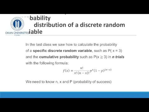
- 3. Probability and cumulative probability distribution of a discrete random variable
- 4. The binomial distribution is used to find the probability of a specific or cumulative number of
- 5. Probability and cumulative probability distribution of a discrete random variable
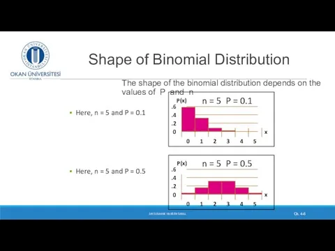
- 6. Ch. 4- DR SUSANNE HANSEN SARAL Shape of Binomial Distribution The shape of the binomial distribution
- 7. Binomial Distribution shapes When P = .5 the shape of the distribution is perfectly symmetrical and
- 8. Using Binomial Tables instead of to calculating Binomial probabilities manually DR SUSANNE HANSEN SARAL Ch. 4-
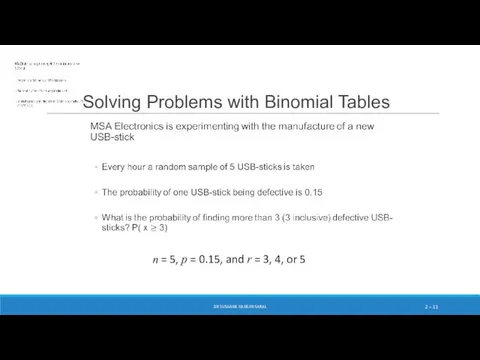
- 9. Solving Problems with Binomial Tables MSA Electronics is experimenting with the manufacture of a new USB-stick
- 10. Solving Problems with Binomial Tables DR SUSANNE HANSEN SARAL 2 – TABLE 2.9 (partial) – Table
- 11. Solving Problems with Binomial Tables DR SUSANNE HANSEN SARAL 2 – n = 5, p =
- 12. Solving Problems with Binomial Tables Cumulative probability DR SUSANNE HANSEN SARAL 2 – TABLE 2.9 (partial)
- 13. Solving Problems with Binomial Tables Cumulative probabilities DR SUSANNE HANSEN SARAL 2 – TABLE 2.9 (partial)
- 14. Suppose that Ali, a real estate agent, has 10 people interested in buying a house. He
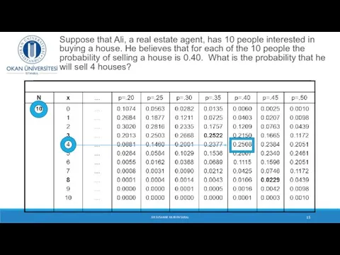
- 15. Suppose that Ali, a real estate agent, has 10 people interested in buying a house. He
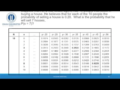
- 16. Suppose that Ali, a real estate agent, has 10 people interested in buying a house. He
- 17. DR SUSANNE HANSEN SARAL
- 18. Probability Distributions Continuous Probability Distributions Binomial Probability Distributions Discrete Probability Distributions Uniform Normal Exponential DR SUSANNE
- 19. Poisson random variable, first proposed by Frenchman Simeon Poisson (1781-1840) DR SUSANNE HANSEN SARAL A Poisson
- 20. Poisson Random Variable - three requirements 1. The number of expected outcomes in one interval of
- 21. Poisson Random Variable - three requirements (continued) 2.The expected (or mean) number of outcomes over any
- 22. Examples of a Poisson Random variable The number of cars arriving at a toll booth in
- 23. Situations where the Poisson distribution is widely used: Capacity planning – time interval Areas of capacity
- 24. Poisson Probability Distribution Poisson Probability Function where: f(x) = probability of x occurrences in an interval
- 25. Example: Drive-up ATM Window Poisson Probability Function: Time Interval Suppose that we are interested in the
- 26. Poisson Probability Function: Time Interval λ = 10/15-minutes, x = 5 We want to know the
- 27. Using Poisson ProbabilityTables DR SUSANNE HANSEN SARAL Ch. 4- Example: Find P(X = 2) if λ
- 28. The shape of a Poisson Probabilities Distribution DR SUSANNE HANSEN SARAL Ch. 4- P(X = 2)
- 29. Poisson Distribution Shape The shape of the Poisson Distribution depends on the parameter λ : DR
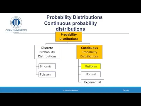
- 30. Probability Distributions Continuous probability distributions Continuous Probability Distributions Binomial Probability Distributions Discrete Probability Distributions Uniform Normal
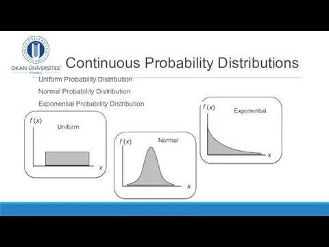
- 31. Continuous Probability Distributions Uniform Probability Distribution Normal Probability Distribution Exponential Probability Distribution f (x) x Uniform
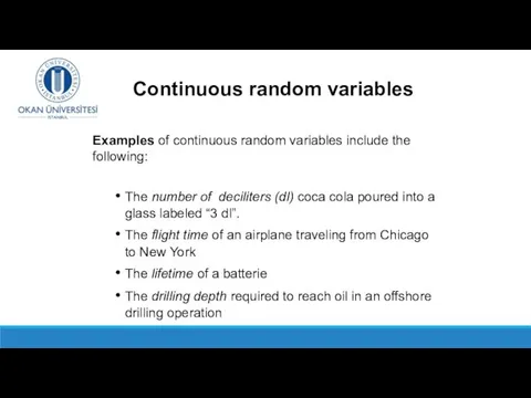
- 32. Examples of continuous random variables include the following: The number of deciliters (dl) coca cola poured
- 33. Continuous random variable A continuous random variable can assume any value in an interval on the
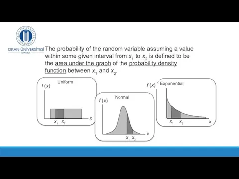
- 34. f (x) x Uniform x f (x) Normal x f (x) Exponential Continuous Probability Distributions The
- 35. Probability Density Function The probability density function, f(x), of a continuous random variable X has the
- 36. Probability Density Function The probability density function, f(x), of random variable X has the following properties:
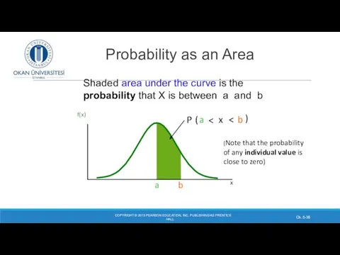
- 37. Probability as an Area COPYRIGHT © 2013 PEARSON EDUCATION, INC. PUBLISHING AS PRENTICE HALL Ch. 5-
- 38. Probability as an Area COPYRIGHT © 2013 PEARSON EDUCATION, INC. PUBLISHING AS PRENTICE HALL Ch. 5-
- 39. Cumulative Distribution Function, F(x) Let a and b be two possible values of X, with a
- 40. Cumulative probability as an Area COPYRIGHT © 2013 PEARSON EDUCATION, INC. PUBLISHING AS PRENTICE HALL Ch.
- 41. Probability Distribution of a Continuous Random Variable Copyright ©2015 Pearson Education, Inc. 2 – FIGURE 2.5
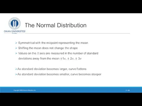
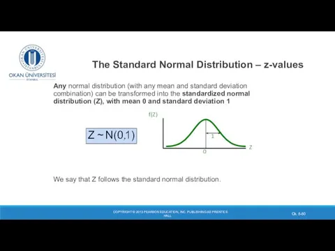
- 42. The Normal Distribution The Normal Distribution is one of the most popular and useful continuous probability
- 43. ‘Bell Shaped’ Symmetrical Mean, Median and Mode are Equal Location of the curve is determined by
- 44. Copyright ©2015 Pearson Education, Inc. 2 – The location of the normal distribution on the x-axis
- 45. Copyright ©2015 Pearson Education, Inc. 2 – The shape of the normal distribution is described by
- 46. The Normal Distribution Copyright ©2015 Pearson Education, Inc. 2 –
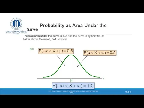
- 47. Probability as Area Under the Curve COPYRIGHT © 2013 PEARSON EDUCATION, INC. PUBLISHING AS PRENTICE HALL
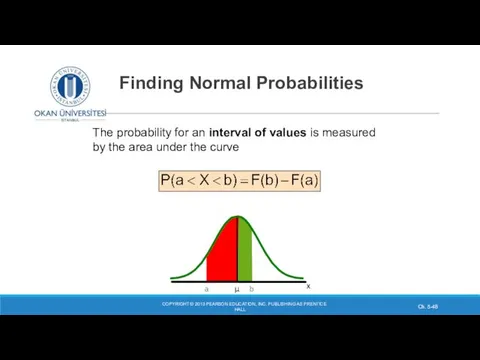
- 48. Finding Normal Probabilities COPYRIGHT © 2013 PEARSON EDUCATION, INC. PUBLISHING AS PRENTICE HALL Ch. 5- x
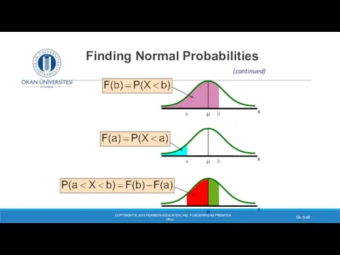
- 49. Finding Normal Probabilities COPYRIGHT © 2013 PEARSON EDUCATION, INC. PUBLISHING AS PRENTICE HALL Ch. 5- x
- 50. COPYRIGHT © 2013 PEARSON EDUCATION, INC. PUBLISHING AS PRENTICE HALL Ch. 5- The Standard Normal Distribution
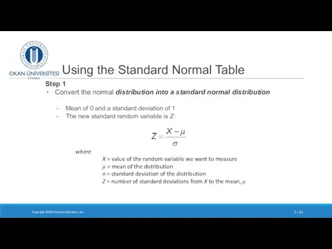
- 51. Using the Standard Normal Table Step 1 Convert the normal distribution into a standard normal distribution
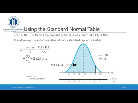
- 52. Using the Standard Normal Table For μ = 100, σ = 15, find the probability that
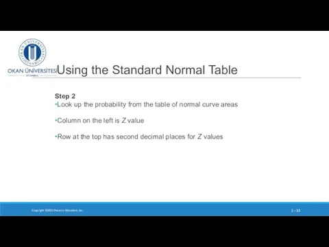
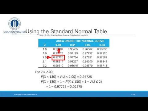
- 53. Using the Standard Normal Table Step 2 Look up the probability from the table of normal
- 54. Using the Standard Normal Table Copyright ©2015 Pearson Education, Inc. 2 – TABLE 2.10 – Standardized
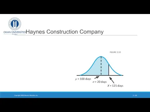
- 55. Haynes Construction Company Copyright ©2015 Pearson Education, Inc. 2 – FIGURE 2.10
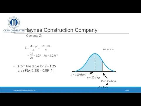
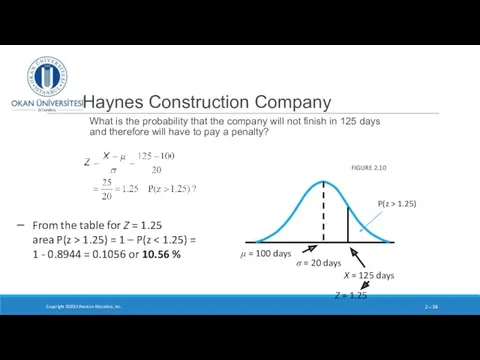
- 56. Haynes Construction Company Compute Z: Copyright ©2015 Pearson Education, Inc. 2 – FIGURE 2.10 From the
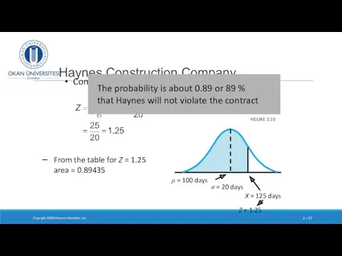
- 57. Compute Z Haynes Construction Company Copyright ©2015 Pearson Education, Inc. 2 – FIGURE 2.10 From the
- 58. Haynes Construction Company What is the probability that the company will not finish in 125 days
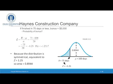
- 59. Haynes Construction Company If finished in 75 days or less, bonus = $5,000 Probability of bonus?
- 60. If finished in 75 days or less, bonus = $5,000 Probability of bonus? Haynes Construction Company
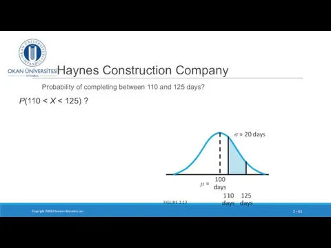
- 61. Haynes Construction Company Probability of completing between 110 and 125 days? Copyright ©2015 Pearson Education, Inc.
- 63. Скачать презентацию
Mid-term exam
23/03/2017 11:45 – 13:00 hours
Bring:
Calculator
Pen
Eraser
Mid-term exam
23/03/2017 11:45 – 13:00 hours
Bring:
Calculator
Pen
Eraser
Probability and cumulative probability distribution of a discrete random variable
Probability and cumulative probability distribution of a discrete random variable
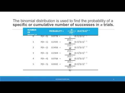
The binomial distribution is used to find the probability of a
The binomial distribution is used to find the probability of a
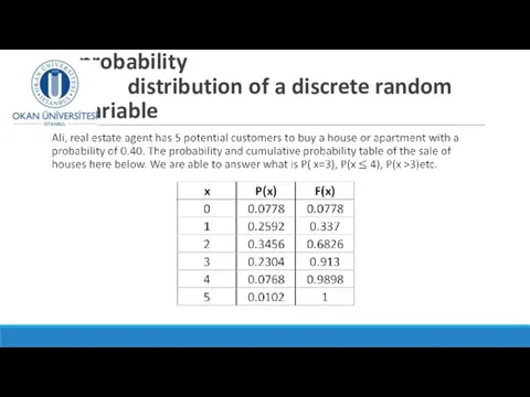
Probability and cumulative probability distribution of a discrete random variable
Probability and cumulative probability distribution of a discrete random variable
Ch. 4-
DR SUSANNE HANSEN SARAL
Shape of Binomial Distribution
The shape of the
Ch. 4-
DR SUSANNE HANSEN SARAL
Shape of Binomial Distribution
The shape of the
Binomial Distribution shapes
When P = .5 the shape of the
Binomial Distribution shapes
When P = .5 the shape of the
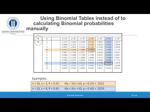
Using Binomial Tables instead of to calculating Binomial probabilities manually
DR
Using Binomial Tables instead of to calculating Binomial probabilities manually
DR
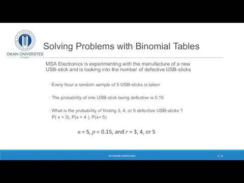
Solving Problems with Binomial Tables
MSA Electronics is experimenting with the manufacture
Solving Problems with Binomial Tables
MSA Electronics is experimenting with the manufacture
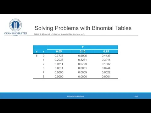
Solving Problems with Binomial Tables
DR SUSANNE HANSEN SARAL
2 –
TABLE
Solving Problems with Binomial Tables
DR SUSANNE HANSEN SARAL
2 –
TABLE
Solving Problems with Binomial Tables
DR SUSANNE HANSEN SARAL
2 –
n =
Solving Problems with Binomial Tables
DR SUSANNE HANSEN SARAL
2 –
n =
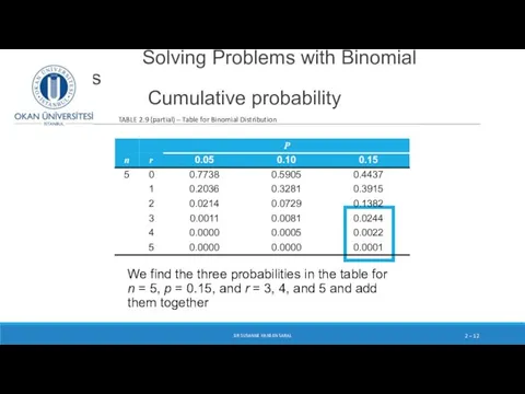
Solving Problems with Binomial Tables
Cumulative probability
DR SUSANNE HANSEN SARAL
2
Solving Problems with Binomial Tables
Cumulative probability
DR SUSANNE HANSEN SARAL
2
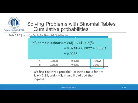
Solving Problems with Binomial Tables
Cumulative probabilities
DR SUSANNE HANSEN SARAL
2
Solving Problems with Binomial Tables
Cumulative probabilities
DR SUSANNE HANSEN SARAL
2
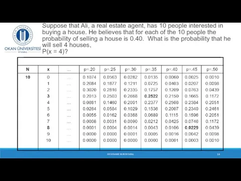
Suppose that Ali, a real estate agent, has 10 people interested
Suppose that Ali, a real estate agent, has 10 people interested
Suppose that Ali, a real estate agent, has 10 people interested
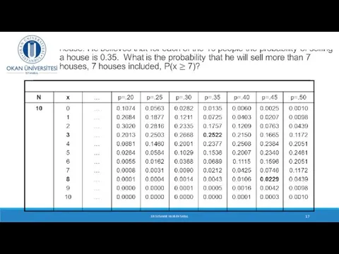
Suppose that Ali, a real estate agent, has 10 people interested
Suppose that Ali, a real estate agent, has 10 people interested
Suppose that Ali, a real estate agent, has 10 people interested
DR SUSANNE HANSEN SARAL
DR SUSANNE HANSEN SARAL
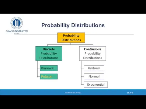
Probability Distributions
Continuous
Probability Distributions
Binomial
Probability Distributions
Discrete
Probability Distributions
Uniform
Normal
Exponential
DR SUSANNE HANSEN SARAL
Ch.
Probability Distributions
Continuous
Probability Distributions
Binomial
Probability Distributions
Discrete
Probability Distributions
Uniform
Normal
Exponential
DR SUSANNE HANSEN SARAL
Ch.
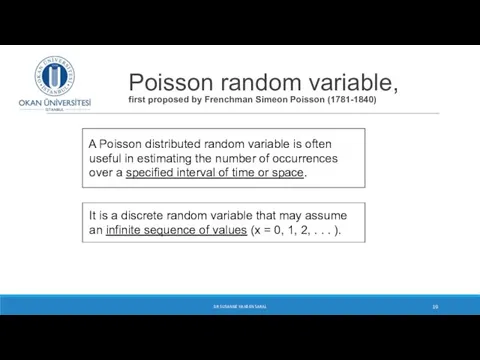
Poisson random variable,
first proposed by Frenchman Simeon Poisson (1781-1840)
DR SUSANNE HANSEN
Poisson random variable,
first proposed by Frenchman Simeon Poisson (1781-1840)
DR SUSANNE HANSEN
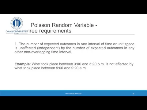
Poisson Random Variable - three requirements
1. The number of expected outcomes
Poisson Random Variable - three requirements
1. The number of expected outcomes
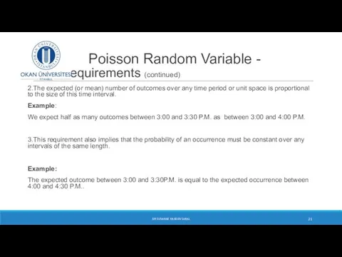
Poisson Random Variable - three requirements (continued)
2.The expected (or mean)
Poisson Random Variable - three requirements (continued)
2.The expected (or mean)
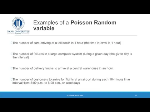
Examples of a Poisson Random variable
The number of cars arriving at
Examples of a Poisson Random variable
The number of cars arriving at
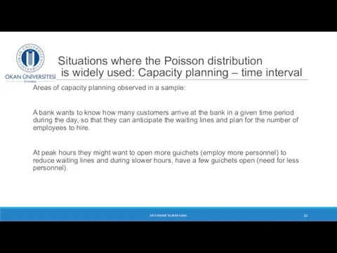
Situations where the Poisson distribution
is widely used: Capacity planning
Situations where the Poisson distribution is widely used: Capacity planning
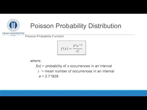
Poisson Probability Distribution
Poisson Probability Function
where:
f(x) = probability of x occurrences
Poisson Probability Distribution
Poisson Probability Function
where:
f(x) = probability of x occurrences
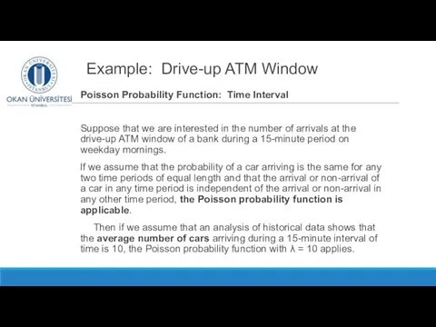
Example: Drive-up ATM Window
Poisson Probability Function: Time Interval
Suppose that we are
Example: Drive-up ATM Window
Poisson Probability Function: Time Interval
Suppose that we are
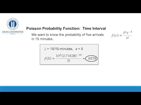
Poisson Probability Function: Time Interval
λ = 10/15-minutes, x = 5
We want
Poisson Probability Function: Time Interval
λ = 10/15-minutes, x = 5
We want
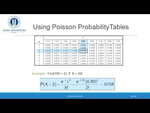
Using Poisson ProbabilityTables
DR SUSANNE HANSEN SARAL
Ch. 4-
Example: Find P(X = 2)
Using Poisson ProbabilityTables
DR SUSANNE HANSEN SARAL
Ch. 4-
Example: Find P(X = 2)
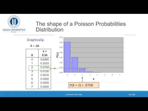
The shape of a Poisson Probabilities Distribution
DR SUSANNE HANSEN SARAL
Ch. 4-
P(X
The shape of a Poisson Probabilities Distribution
DR SUSANNE HANSEN SARAL
Ch. 4-
P(X
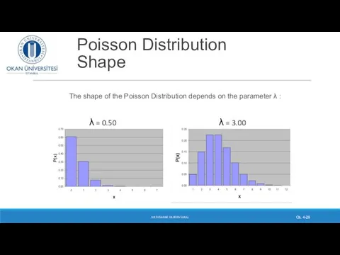
Poisson Distribution Shape
The shape of the Poisson Distribution depends on the
Poisson Distribution Shape
The shape of the Poisson Distribution depends on the
Probability Distributions Continuous probability distributions
Continuous
Probability Distributions
Binomial
Probability Distributions
Discrete
Probability
Probability Distributions Continuous probability distributions
Continuous
Probability Distributions
Binomial
Probability Distributions
Discrete
Probability
Continuous Probability Distributions
Uniform Probability Distribution
Normal Probability Distribution
Exponential Probability Distribution
f (x)
x
Uniform
x
f
Continuous Probability Distributions
Uniform Probability Distribution
Normal Probability Distribution
Exponential Probability Distribution
f (x)
x
Uniform
x
f
Examples of continuous random variables include the following:
The number of
Examples of continuous random variables include the following:
The number of
Continuous random variable
A continuous random variable can assume any value in
Continuous random variable
A continuous random variable can assume any value in
f (x)
x
Uniform
x
f (x)
Normal
x
f (x)
Exponential
Continuous Probability Distributions
The probability of the random
f (x)
x
Uniform
x
f (x)
Normal
x
f (x)
Exponential
Continuous Probability Distributions
The probability of the random
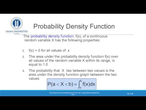
Probability Density Function
The probability density function, f(x), of a continuous random
Probability Density Function
The probability density function, f(x), of a continuous random
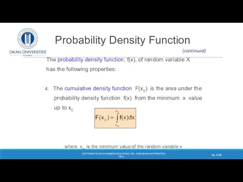
Probability Density Function
The probability density function, f(x), of random variable X
has
Probability Density Function
The probability density function, f(x), of random variable X
has
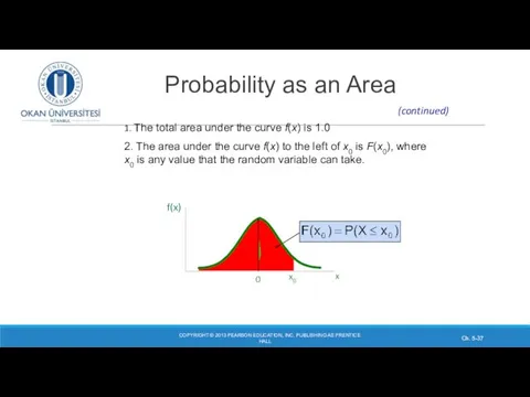
Probability as an Area
COPYRIGHT © 2013 PEARSON EDUCATION, INC.
Probability as an Area
COPYRIGHT © 2013 PEARSON EDUCATION, INC.
Probability as an Area
COPYRIGHT © 2013 PEARSON EDUCATION, INC.
Probability as an Area
COPYRIGHT © 2013 PEARSON EDUCATION, INC.
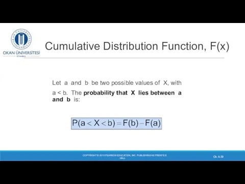
Cumulative Distribution Function, F(x)
Let a and b be two possible
Cumulative Distribution Function, F(x)
Let a and b be two possible
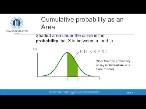
Cumulative probability as an Area
COPYRIGHT © 2013 PEARSON EDUCATION,
Cumulative probability as an Area
COPYRIGHT © 2013 PEARSON EDUCATION,
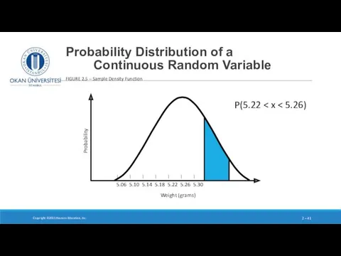
Probability Distribution of a Continuous Random Variable
Copyright ©2015 Pearson Education,
Probability Distribution of a Continuous Random Variable
Copyright ©2015 Pearson Education,
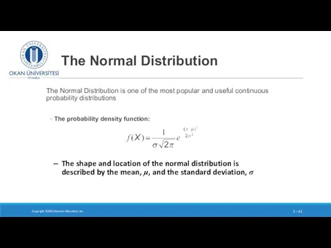
The Normal Distribution
The Normal Distribution is one of the most popular
The Normal Distribution
The Normal Distribution is one of the most popular
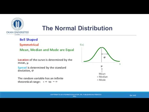
‘Bell Shaped’
Symmetrical
Mean, Median and Mode are Equal
Location
‘Bell Shaped’
Symmetrical
Mean, Median and Mode are Equal
Location
Copyright ©2015 Pearson Education, Inc.
2 –
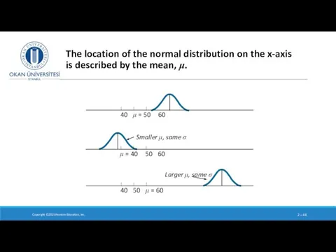
The location of the normal
Copyright ©2015 Pearson Education, Inc.
2 –
The location of the normal
Copyright ©2015 Pearson Education, Inc.
2 –
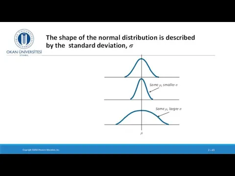
The shape of the normal
Copyright ©2015 Pearson Education, Inc.
2 –
The shape of the normal
The Normal Distribution
Copyright ©2015 Pearson Education, Inc.
2 –
The Normal Distribution
Copyright ©2015 Pearson Education, Inc.
2 –
Probability as Area Under the Curve
COPYRIGHT © 2013 PEARSON
Probability as Area Under the Curve
COPYRIGHT © 2013 PEARSON
Finding Normal Probabilities
COPYRIGHT © 2013 PEARSON EDUCATION, INC.
Finding Normal Probabilities
COPYRIGHT © 2013 PEARSON EDUCATION, INC.
Finding Normal Probabilities
COPYRIGHT © 2013 PEARSON EDUCATION, INC.
Finding Normal Probabilities
COPYRIGHT © 2013 PEARSON EDUCATION, INC.
COPYRIGHT © 2013 PEARSON EDUCATION, INC. PUBLISHING AS PRENTICE HALL
Ch.
COPYRIGHT © 2013 PEARSON EDUCATION, INC. PUBLISHING AS PRENTICE HALL
Ch.
Using the Standard Normal Table
Step 1
Convert the normal distribution into
Using the Standard Normal Table
Step 1
Convert the normal distribution into
Using the Standard Normal Table
For μ = 100, σ = 15,
Using the Standard Normal Table
For μ = 100, σ = 15,
Using the Standard Normal Table
Step 2
Look up the probability from the
Using the Standard Normal Table
Step 2
Look up the probability from the
Using the Standard Normal Table
Copyright ©2015 Pearson Education, Inc.
2 –
TABLE
Using the Standard Normal Table
Copyright ©2015 Pearson Education, Inc.
2 –
TABLE
Haynes Construction Company
Copyright ©2015 Pearson Education, Inc.
2 –
FIGURE 2.10
Haynes Construction Company
Copyright ©2015 Pearson Education, Inc.
2 –
FIGURE 2.10
Haynes Construction Company
Compute Z:
Copyright ©2015 Pearson Education, Inc.
2 –
FIGURE
Haynes Construction Company
Compute Z:
Copyright ©2015 Pearson Education, Inc.
2 –
FIGURE
Compute Z
Haynes Construction Company
Copyright ©2015 Pearson Education, Inc.
2 –
FIGURE
Compute Z
Haynes Construction Company
Copyright ©2015 Pearson Education, Inc.
2 –
FIGURE
Haynes Construction Company
What is the probability that the company will
Haynes Construction Company
What is the probability that the company will
Haynes Construction Company
If finished in 75 days or less, bonus
Haynes Construction Company
If finished in 75 days or less, bonus
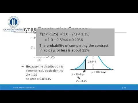
If finished in 75 days or less, bonus = $5,000
Probability of
If finished in 75 days or less, bonus = $5,000
Probability of
Haynes Construction Company
Probability of completing between 110 and 125 days?
Copyright
Haynes Construction Company
Probability of completing between 110 and 125 days?
Copyright
 Методика обучения математике в начальной школе как педагогическая наука. Лекция 1
 Степень с целым показателем. 8 класс
 Решение задач с помощью систем уравнений
 Генеральная совокупность и частотное распределение. Измерение связи между качественными переменными
 Измерение углов. Транспортир. 5 класс
 Делимость чисел. Обобщение знаний
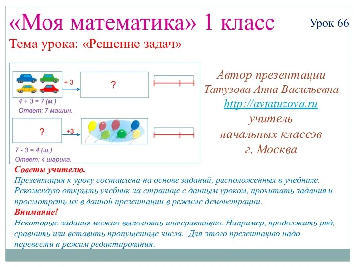 Математика. 1 класс. Урок 66. Решение задач - Презентация
 Равнобедренный треугольник. Свойства равнобедренного треугольника. 7 класс
 Множественный корреляционный анализ
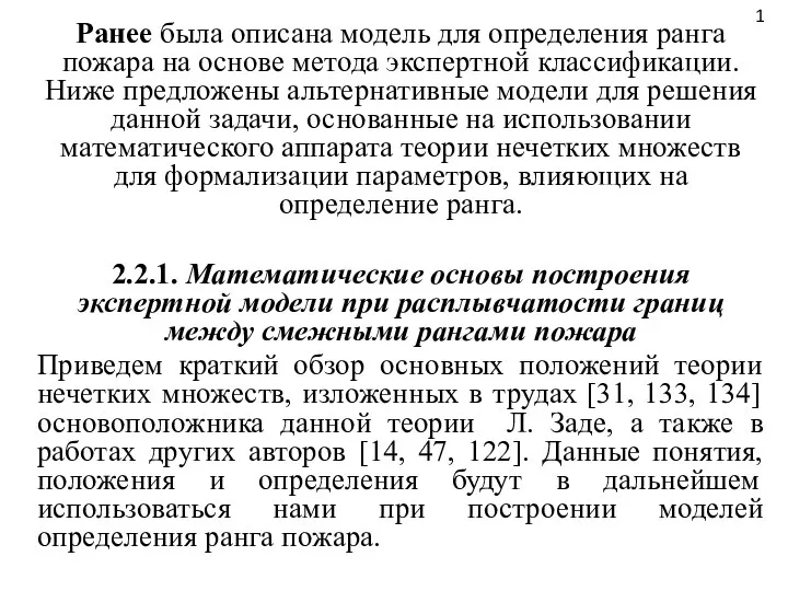 Математические основы построения экспертной модели при расплывчатости границ между смежными рангами пожара
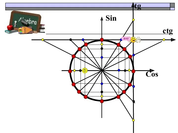 Преобразование графиков тригонометрических функций
 Конспект урока по математике 2 класс УМК Петерсон Л.Г. Свойства сложения + презентация
 Сложение и вычитание в пределах 10. Задачи в стихах.
 Закрепление навыков решения квадратных уравнений. Формирование у учащихся умения решать биквадратные уравнения. 8 класс
 Решение иррациональных уравнений
 Решение примеров и задач на сложение и вычитание в пределах 20.
 Величины. Классная работа
 Призма, пирамида. Понятие и чертёж
 Площадь фигур. Сравнение площадей
 Критерии для принятия решений. Теория игр
 Геометрические фигуры. Отрезок. Длина отрезка
 Связь между суммой и слагаемыми
 Уравнение окружности
 Прикладная статистика. Меры центральной тенденции. Меры разброса. Нормальное распределение
 Бесконечные периодические десятичные дроби
 Архитектурная комбинаторика. Курс лекций
 Зачет по теме Квадратные уравнения
 Длина окружности и площадь круга