- Modelling with Exponentials and Logarithms

Содержание
- 2. Lecture Outline Graphs of transformed Exponential functions Graphs of transformed Logarithmic functions Mathematical modelling Exponential Growth
- 3. Mathematical models Modelling using Exponents and Logarithms Often data does not fit to a linear or
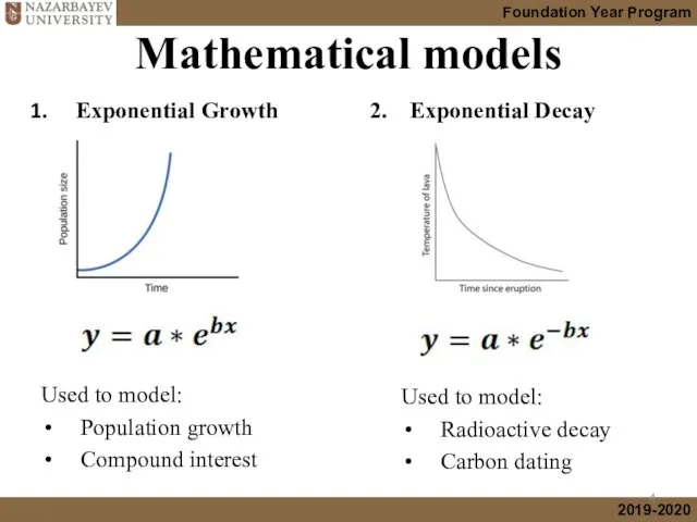
- 4. Mathematical models Exponential Growth Used to model: Population growth Compound interest 2. Exponential Decay Used to
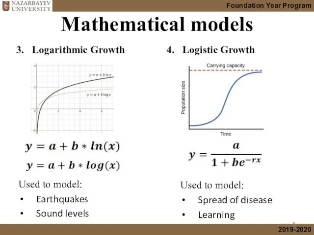
- 5. Mathematical models 3. Logarithmic Growth Used to model: Earthquakes Sound levels 4. Logistic Growth Used to
- 6. Mathematical models 5. Gaussian distribution (Normal distrib.) Used to model: Probability distribution Standardized test (SAT) marks
- 7. Mathematical models Exponential Growth Exponential Decay Logarithmic Model Logistic Growth Gaussian Distribution (Normal Distribution) Note: In
- 8. Introduction to “e” Mathematical constant e is a real, irrational and transcendental number approximately equal to:
- 9. “e” is almost everywhere The logarithmic spiral is a shape that appears in nature, and is
- 10. 2.2.1 Sketch graphs of transformed exponential functions Vertical translation Vertical scaling factor, scale factor b Horizontal
- 11. Let us see some examples:
- 12. Are there any Asymptotes? y=ex Let us see some examples:
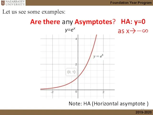
- 13. Are there any Asymptotes? y=ex Let us see some examples: Note: HA (Horizontal asymptote )
- 14. Vertical translation
- 15. Vertical stretch
- 16. Horizontal translation
- 17. Horizontal stretch
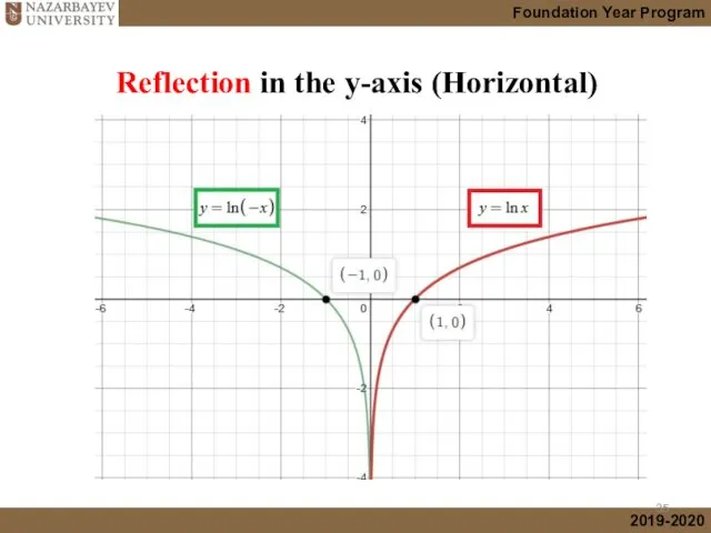
- 18. Reflection in the y-axis (Horizontal)
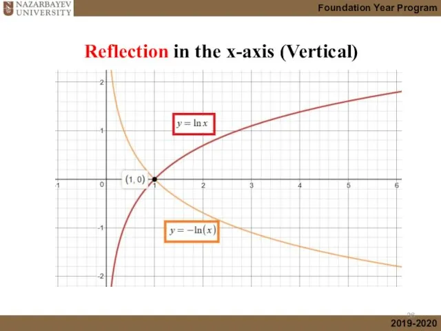
- 19. Reflection in the x-axis (Vertical)
- 20. 1. y=ex 2. y=e2x 3. y=3+e2x (graphs with different scales) Your turn! Match function with its
- 21. 1. y=ex 2. y=e2x 3. y=3+e2x (graphs with different scales) Your turn! Match function with its
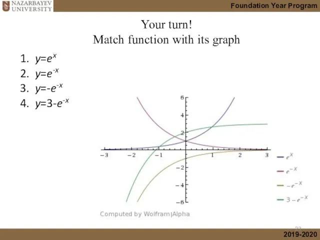
- 22. 1. y=ex 2. y=e-x 3. y=-e-x 4. y=3-e-x Your turn! Match function with its graph
- 23. 1. y=ex 2. y=e-x 3. y=-e-x 4. y=3-e-x Your turn! Match function with its graph
- 24. Have you noticed that we are now dealing with only base “e”? What is the reason
- 25. 1. How to relate 2x to ex 2. What kind of transformation should be applied to
- 26. Answer: we need to apply horizontal stretch, i.e. and introduce a coefficient c 2x = ecx
- 27. 2x = exln2
- 28. That is why in Exponential growth and decay models we use directly “e” number that can
- 29. 2.2.2 Sketch graphs of transformed natural logarithmic functions Vertical translation Vertical scaling factor, scale factor b
- 30. Let us see some examples:
- 31. Vertical translation Are there any Asymptotes? Note: VA (Vertical asymptote )
- 32. Vertical stretch
- 33. Horizontal translation Asymptotes
- 34. Horizontal stretch
- 35. Reflection in the y-axis (Horizontal)
- 36. Reflection in the x-axis (Vertical)
- 37. 1. y=lnx 2. y=ln(-x) 3. y=ln(3-x) 4. y=-ln(3-x) 5. y=2-ln(3-x) Let us see some examples:
- 38. 1. y=lnx 2. y=ln(2x) 3. y=2+ln(2x) Your turn! Match function with its graph
- 39. 2.2.3 Interpret and perform calculations with Exponential Growth and Decay models Exponential Growth Exponential Decay Note
- 40. Example 1 Decay model The new price The value at 5 years old car What the
- 41. Solutions:
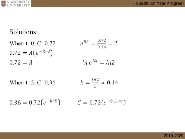
- 42. Your turn (Example 2 Growth model) The exponential growth of a colony of bacteria can modeled
- 43. a. Initial population A= 60e0.03(0)=60e0=60 bacteria Solutions: A=60e(0.03t) c. After what time t will the number
- 45. d.
- 49. 2.2.4 Solve applications involving Exponential and Logarithmic functions Example 5 (Law of forgetting)
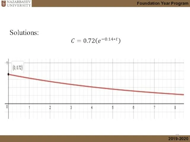
- 50. Solutions:
- 51. Example 6 (Magnitude of earthquake)
- 52. Solutions:
- 53. Your turn (Example 7)
- 54. Solutions:
- 55. Learning outcomes At the end of this lecture, you should be able to: 2.2.1 Sketch the
- 56. Foundation Year Program Preview activity 1: Trigonometry Watch this video https://www.youtube.com/watch?v=T9lt6MZKLck
- 58. Скачать презентацию
Lecture Outline
Graphs of transformed Exponential functions
Graphs of transformed Logarithmic functions
Mathematical modelling
Exponential
Lecture Outline
Graphs of transformed Exponential functions
Graphs of transformed Logarithmic functions
Mathematical modelling
Exponential
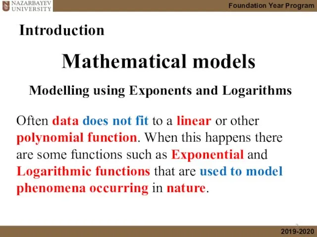
Mathematical models
Modelling using Exponents and Logarithms
Often data does not fit to
Mathematical models
Modelling using Exponents and Logarithms
Often data does not fit to
Mathematical models
Exponential Growth
Used to model:
Population growth
Compound interest
2. Exponential Decay
Used to model:
Radioactive
Mathematical models
Exponential Growth
Used to model:
Population growth
Compound interest
2. Exponential Decay
Used to model:
Radioactive
Mathematical models
3. Logarithmic Growth
Used to model:
Earthquakes
Sound levels
4. Logistic Growth
Used to model:
Spread
Mathematical models
3. Logarithmic Growth
Used to model:
Earthquakes
Sound levels
4. Logistic Growth
Used to model:
Spread
Mathematical models
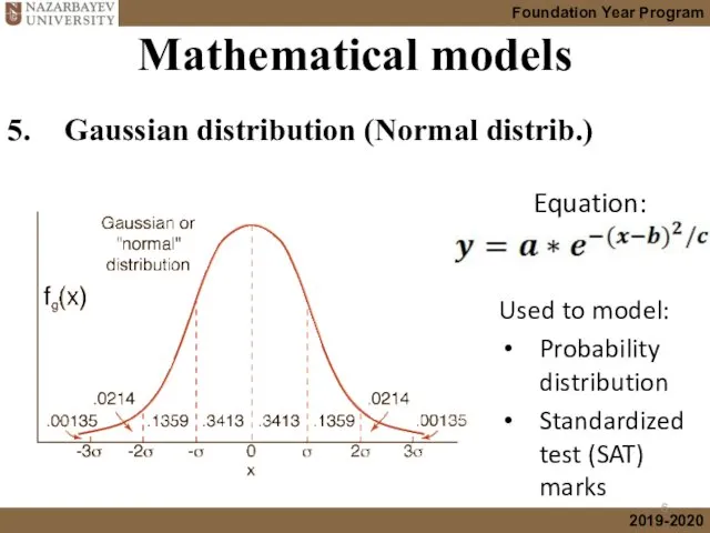
5. Gaussian distribution (Normal distrib.)
Used to model:
Probability distribution
Standardized test (SAT) marks
Equation:
Mathematical models
5. Gaussian distribution (Normal distrib.)
Used to model:
Probability distribution
Standardized test (SAT) marks
Equation:
Mathematical models
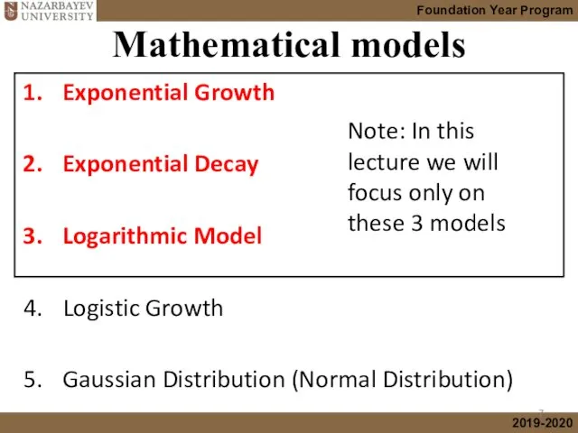
Exponential Growth
Exponential Decay
Logarithmic Model
Logistic Growth
Gaussian Distribution (Normal Distribution)
Note: In
Mathematical models
Exponential Growth
Exponential Decay
Logarithmic Model
Logistic Growth
Gaussian Distribution (Normal Distribution)
Note: In
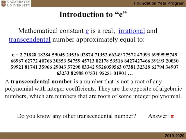
Introduction to “e”
Mathematical constant e is a real, irrational and transcendental
Introduction to “e”
Mathematical constant e is a real, irrational and transcendental
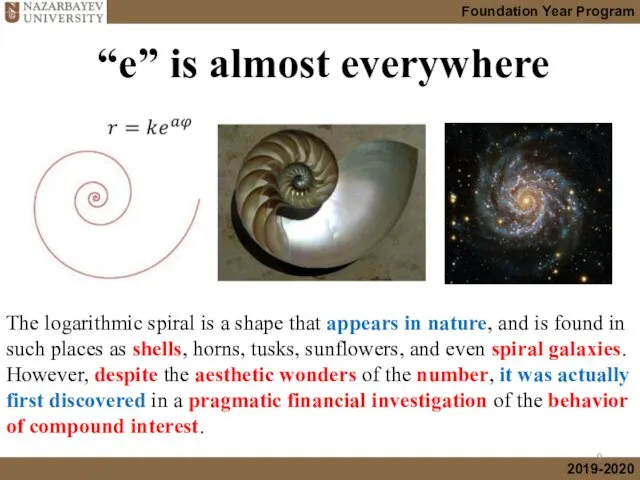
“e” is almost everywhere
The logarithmic spiral is a shape that appears
“e” is almost everywhere
The logarithmic spiral is a shape that appears
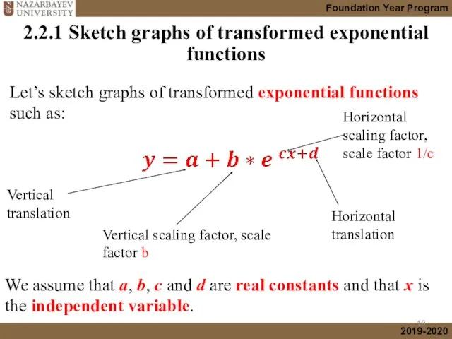
2.2.1 Sketch graphs of transformed exponential functions
Vertical
translation
Vertical scaling factor, scale
2.2.1 Sketch graphs of transformed exponential functions
Vertical
translation
Vertical scaling factor, scale
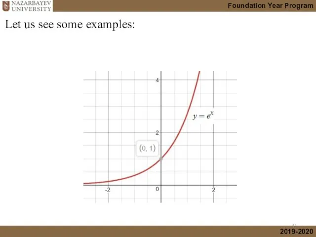
Let us see some examples:
Let us see some examples:
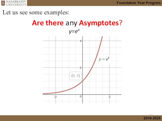
Are there any Asymptotes?
y=ex
Let us see some examples:
Are there any Asymptotes?
y=ex
Let us see some examples:
Are there any Asymptotes?
y=ex
Let us see some examples:
Note: HA (Horizontal
Are there any Asymptotes?
y=ex
Let us see some examples:
Note: HA (Horizontal
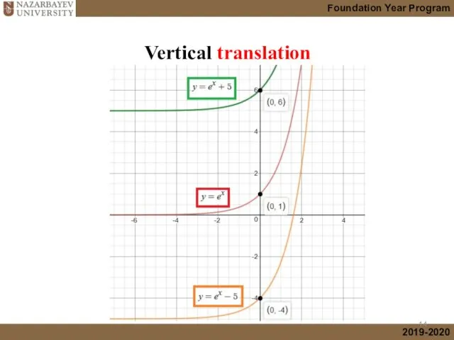
Vertical translation
Vertical translation
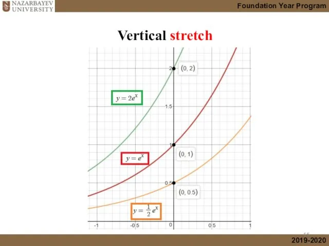
Vertical stretch
Vertical stretch
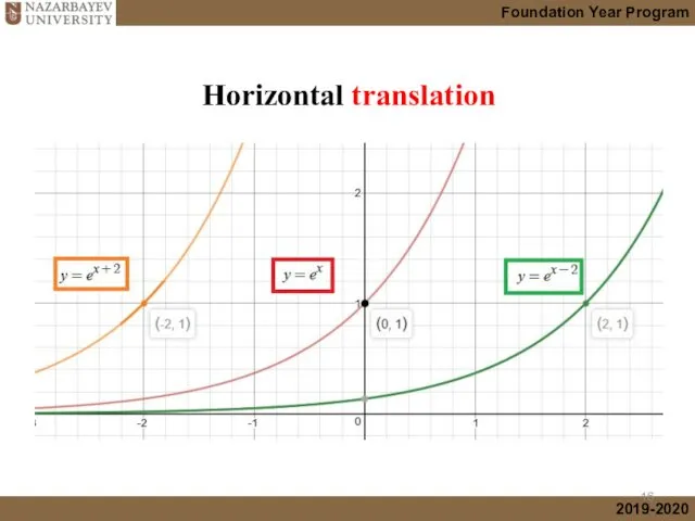
Horizontal translation
Horizontal translation
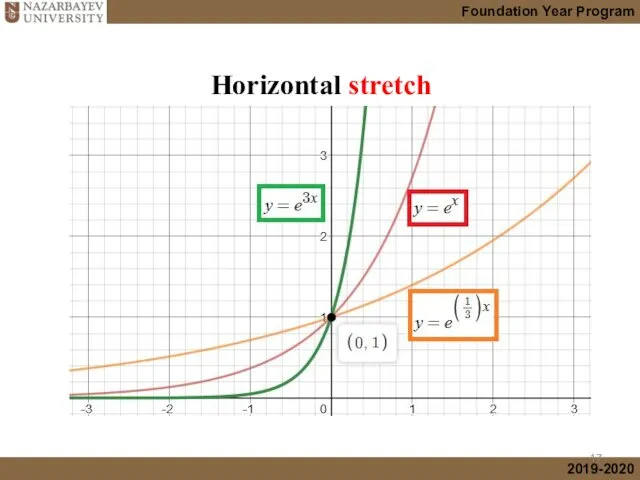
Horizontal stretch
Horizontal stretch
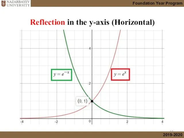
Reflection in the y-axis (Horizontal)
Reflection in the y-axis (Horizontal)
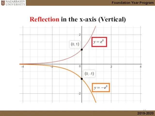
Reflection in the x-axis (Vertical)
Reflection in the x-axis (Vertical)
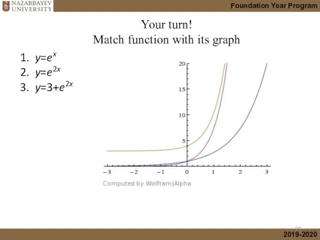
1. y=ex
2. y=e2x
3. y=3+e2x
(graphs with different scales)
Your turn!
Match function with
1. y=ex
2. y=e2x
3. y=3+e2x
(graphs with different scales)
Your turn!
Match function with

1. y=ex
2. y=e2x
3. y=3+e2x
(graphs with different scales)
Your turn!
Match function with
1. y=ex
2. y=e2x
3. y=3+e2x
(graphs with different scales)
Your turn!
Match function with
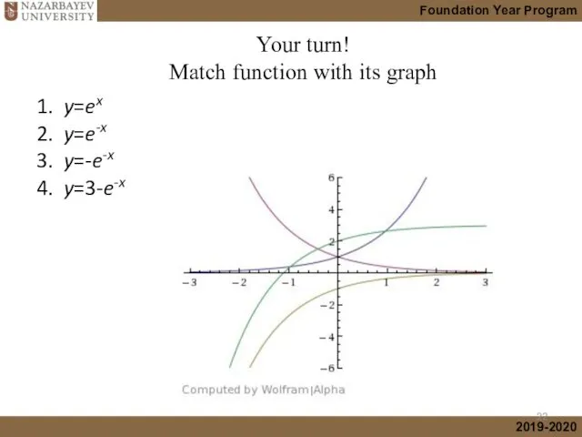
1. y=ex
2. y=e-x
3. y=-e-x
4. y=3-e-x
Your turn!
Match function with its graph
1. y=ex
2. y=e-x
3. y=-e-x
4. y=3-e-x
Your turn!
Match function with its graph
1. y=ex
2. y=e-x
3. y=-e-x
4. y=3-e-x
Your turn!
Match function with its graph
1. y=ex
2. y=e-x
3. y=-e-x
4. y=3-e-x
Your turn!
Match function with its graph
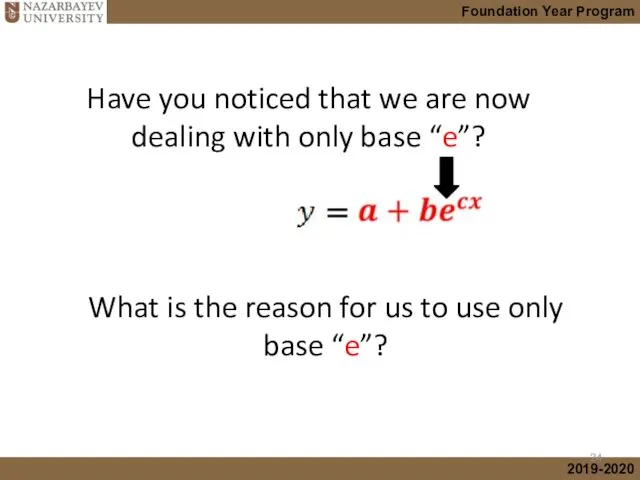
Have you noticed that we are now dealing with only base
Have you noticed that we are now dealing with only base
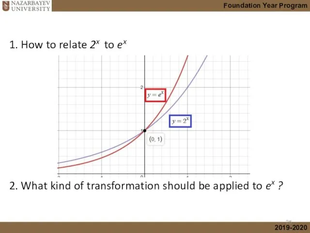
1. How to relate 2x to ex
2. What kind of
1. How to relate 2x to ex
2. What kind of
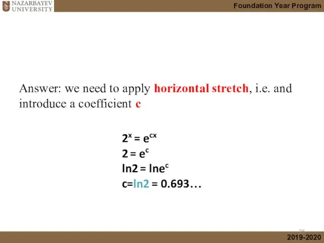
Answer: we need to apply horizontal stretch, i.e. and introduce a
Answer: we need to apply horizontal stretch, i.e. and introduce a
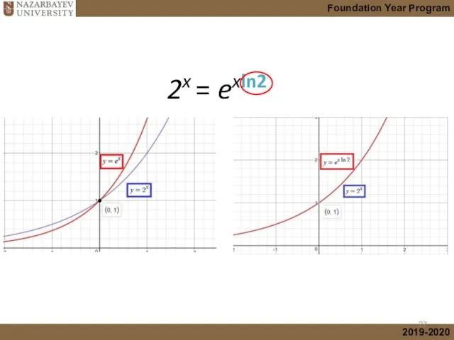
2x = exln2
2x = exln2
That is why in Exponential growth and decay models we use
That is why in Exponential growth and decay models we use
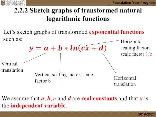
2.2.2 Sketch graphs of transformed natural logarithmic functions
Vertical
translation
Vertical scaling factor,
2.2.2 Sketch graphs of transformed natural logarithmic functions
Vertical
translation
Vertical scaling factor,
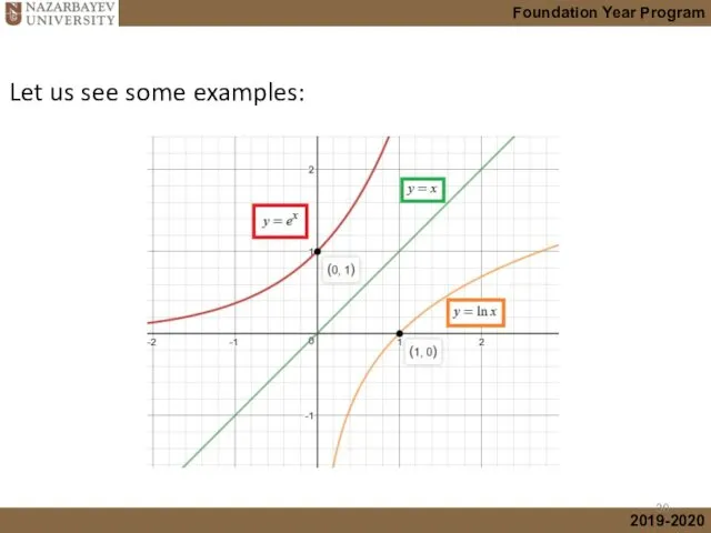
Let us see some examples:
Let us see some examples:
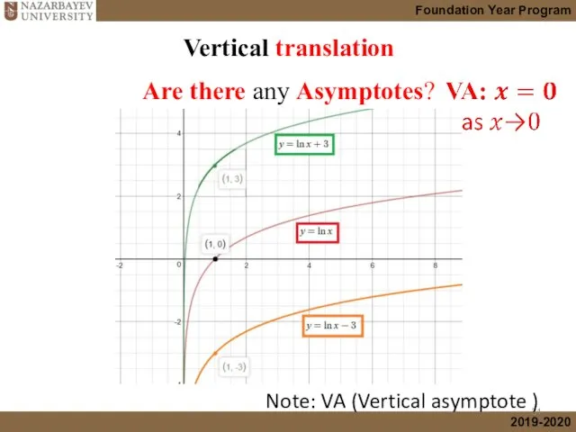
Vertical translation
Are there any Asymptotes?
Note: VA (Vertical asymptote )
Vertical translation
Are there any Asymptotes?
Note: VA (Vertical asymptote )
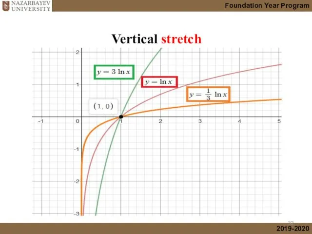
Vertical stretch
Vertical stretch
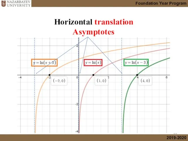
Horizontal translation
Asymptotes
Horizontal translation
Asymptotes
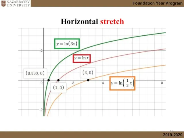
Horizontal stretch
Horizontal stretch
Reflection in the y-axis (Horizontal)
Reflection in the y-axis (Horizontal)
Reflection in the x-axis (Vertical)
Reflection in the x-axis (Vertical)
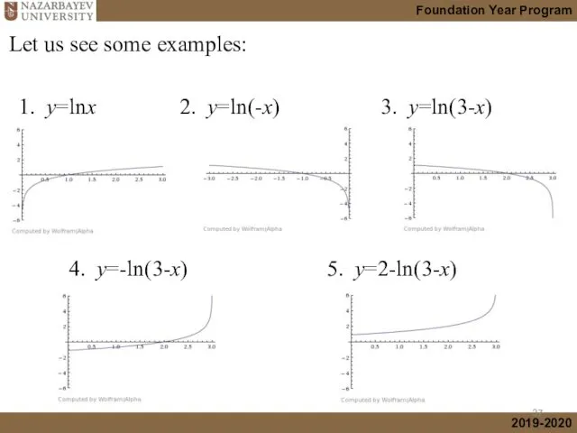
1. y=lnx 2. y=ln(-x) 3. y=ln(3-x)
4. y=-ln(3-x) 5. y=2-ln(3-x)
Let us see
4. y=-ln(3-x) 5. y=2-ln(3-x)
Let us see
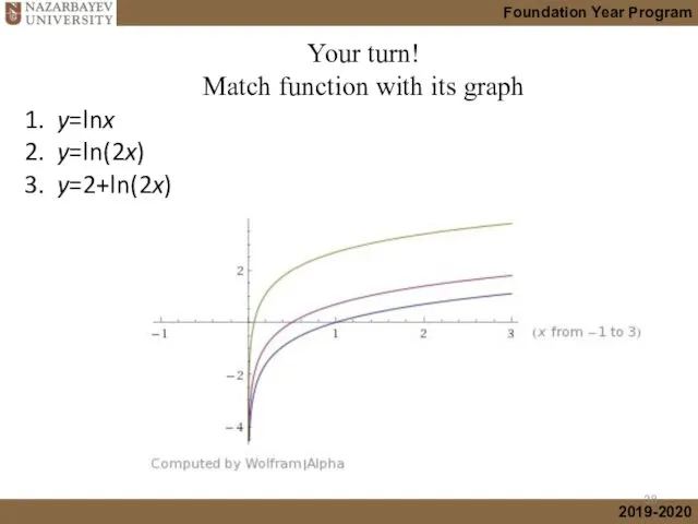
1. y=lnx
2. y=ln(2x)
3. y=2+ln(2x)
Your turn!
Match function with its graph
1. y=lnx
2. y=ln(2x)
3. y=2+ln(2x)
Your turn!
Match function with its graph
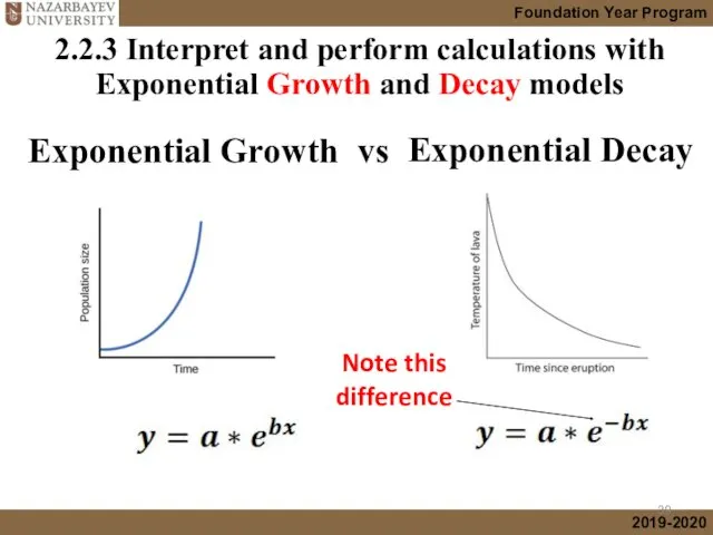
2.2.3 Interpret and perform calculations with Exponential Growth and Decay models
Exponential
2.2.3 Interpret and perform calculations with Exponential Growth and Decay models
Exponential
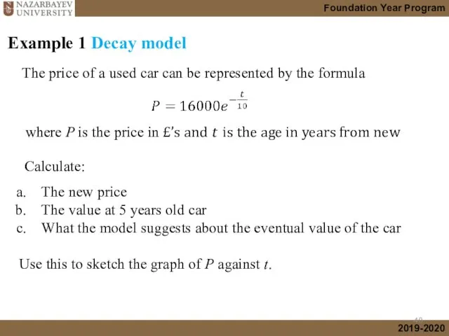
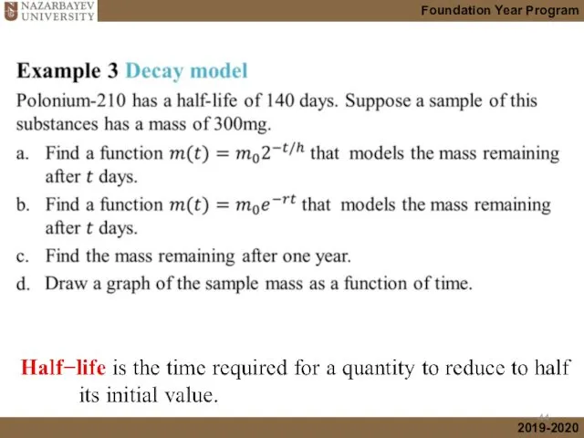
Example 1 Decay model
The new price
The value at 5 years
Example 1 Decay model
The new price
The value at 5 years
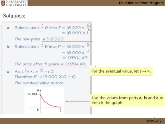
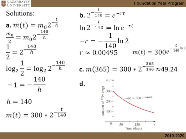
Solutions:
Solutions:
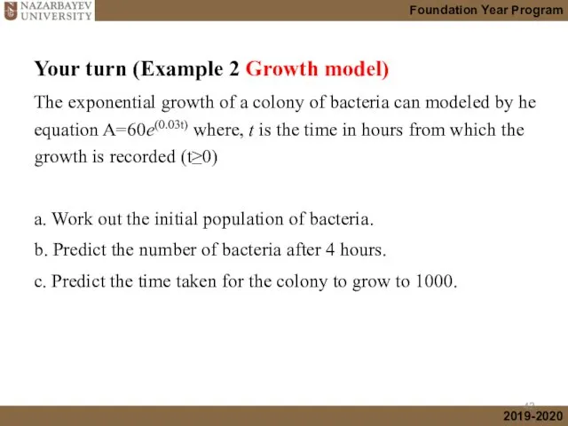
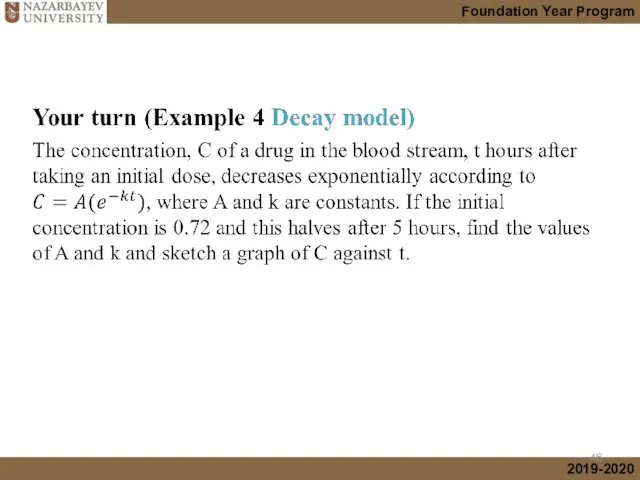
Your turn (Example 2 Growth model)
The exponential growth of a
Your turn (Example 2 Growth model)
The exponential growth of a
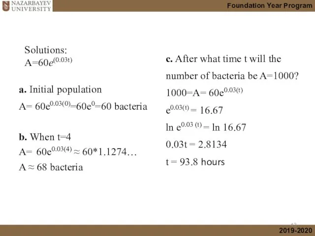
a. Initial population
A= 60e0.03(0)=60e0=60 bacteria
Solutions:
A=60e(0.03t)
c. After what time t will
a. Initial population
A= 60e0.03(0)=60e0=60 bacteria
Solutions:
A=60e(0.03t)
c. After what time t will
d.
d.
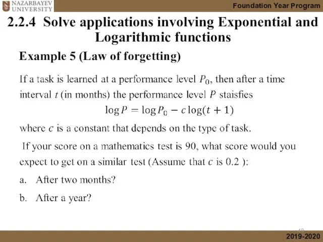
2.2.4 Solve applications involving Exponential and Logarithmic functions
Example 5 (Law of
2.2.4 Solve applications involving Exponential and Logarithmic functions
Example 5 (Law of
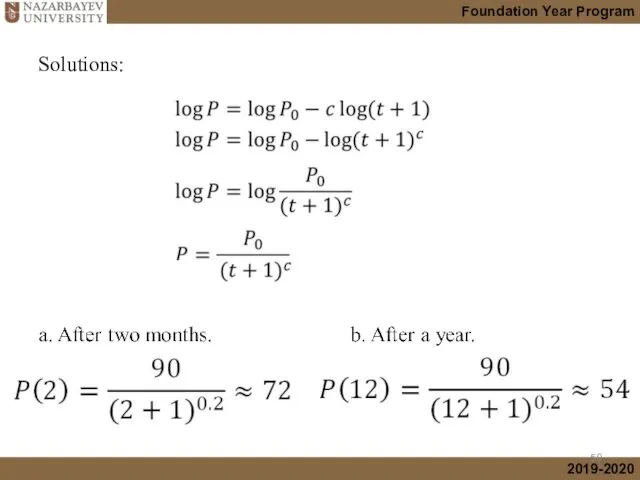
Solutions:
Solutions:
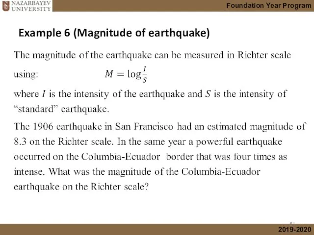
Example 6 (Magnitude of earthquake)
Example 6 (Magnitude of earthquake)
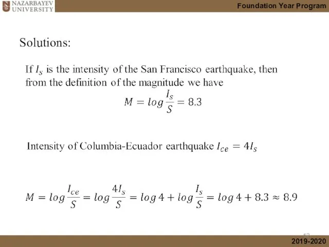
Solutions:
Solutions:
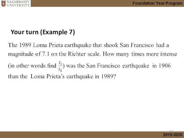
Your turn (Example 7)
Your turn (Example 7)
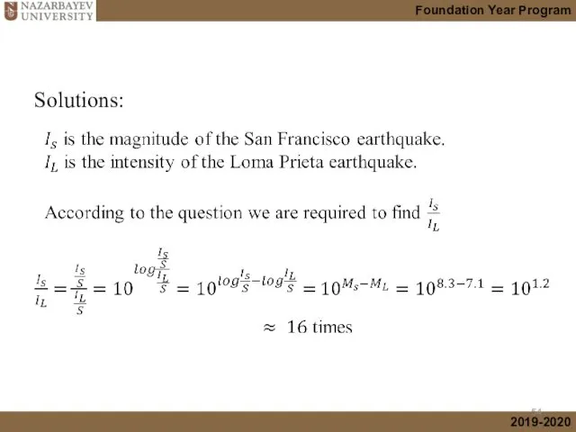
Solutions:
Solutions:
Learning outcomes
At the end of this lecture, you should be able
Learning outcomes
At the end of this lecture, you should be able
Foundation Year Program
Preview activity 1: Trigonometry
Watch this video
https://www.youtube.com/watch?v=T9lt6MZKLck
Foundation Year Program
Preview activity 1: Trigonometry
Watch this video
https://www.youtube.com/watch?v=T9lt6MZKLck
 Деление на десятичную дробь
 Вписанная и описанная окружности. Часть 1. 8 класс
 Основные математические положения, применяемые для анализа и построения статистической модели
 Сложение и вычитание одночленов
 Арифметические действия (повторение)
 Методы кибернетики
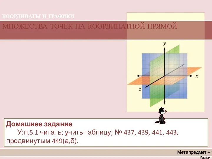 Множества точек на координатной прямой
 Математика в жизни моей семьи
 По сказочной стране Геометрии (конспект с презентацией)
 Нахождение дроби от числа
 Решение задач №19. Проценты
 Тест по математике
 Выпуклый анализ. Выпуклые множества. Лекция 5
 Теріс сандарды қосу
 Тени. Общие положения. Чертежи пространственных фигур. (Лекция 12)
 Масштаб. Решение задач
 Математика в средневековой Индии
 Графический способ решения уравнений
 Знакомство с задачами
 Движение
 Весёлая математика. Задачи в стихах
 сумма трёх и более слагаемых
 Прямые. Взаимное расположение прямых в пространстве. Признак скрещивающихся прямых
 Элементы стереометрии
 Предел функции в бесконечности
 Уменьшаемое, вычитаемое, разность
 Случайные события. Вероятность события
 Задачи на построение сечений. 10 класс