- Object tracking using particle filter

Содержание
- 2. Overview Background Information Basic Particle Filter Theory Rao Blackwellised Particle Filter Color Based Probabilistic Tracking
- 3. Object Tracking Tracking objects in video involves the modeling of non-linear and non-gaussian systems. Non-Linear Non-Gaussian
- 4. Background In order to model accurately the underlying dynamics of a physical system, it is important
- 5. The Particle Filter Particle Filter is concerned with the problem of tracking single and multiple objects.
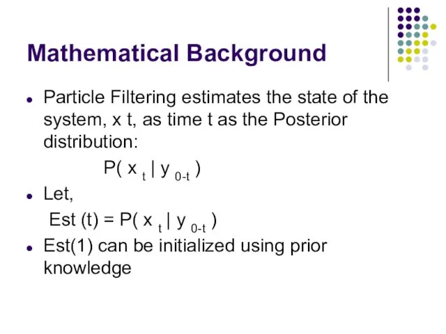
- 6. Mathematical Background Particle Filtering estimates the state of the system, x t, as time t as
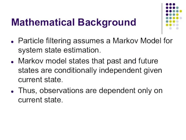
- 7. Mathematical Background Particle filtering assumes a Markov Model for system state estimation. Markov model states that
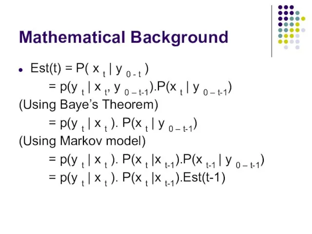
- 8. Mathematical Background Est(t) = P( x t | y 0 - t ) = p(y t
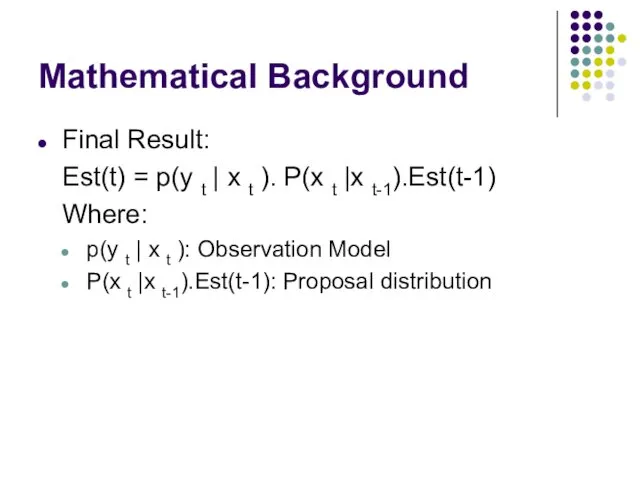
- 9. Mathematical Background Final Result: Est(t) = p(y t | x t ). P(x t |x t-1).Est(t-1)
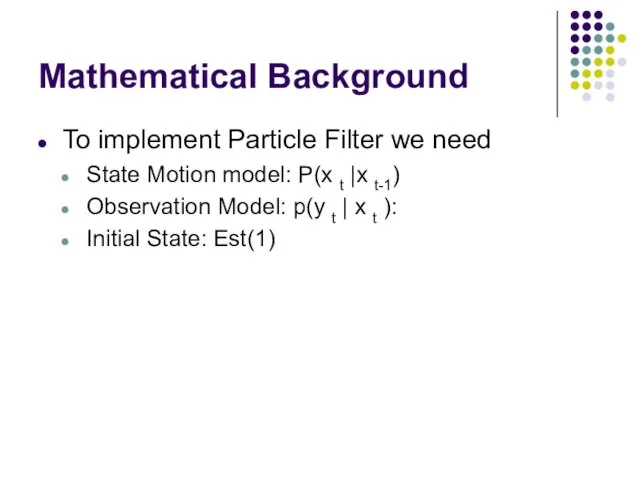
- 10. Mathematical Background To implement Particle Filter we need State Motion model: P(x t |x t-1) Observation
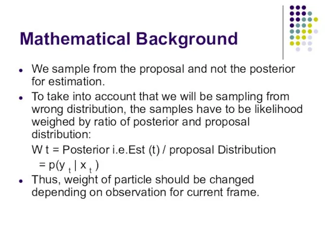
- 11. Mathematical Background We sample from the proposal and not the posterior for estimation. To take into
- 12. Basic Particle Filter Theory A discrete set of samples or particles represents the object-state and evolves
- 13. Basic Particle Filter Theory (Cont.) Particle Filter is concerned with the estimation of the distribution of
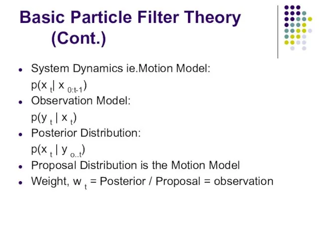
- 14. Basic Particle Filter Theory (Cont.) System Dynamics ie.Motion Model: p(x t| x 0:t-1) Observation Model: p(y
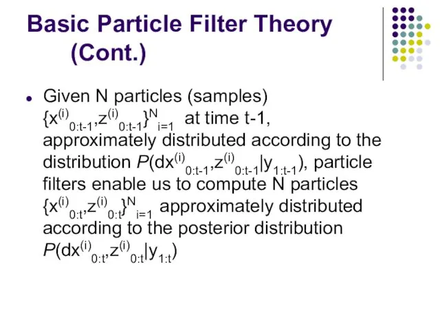
- 15. Basic Particle Filter Theory (Cont.) Given N particles (samples) {x(i)0:t-1,z(i)0:t-1}Ni=1 at time t-1, approximately distributed according
- 16. Basic Particle Filter Theory (Cont.) The basic Particle Filter algorithm consists of 2 steps: Sequential importance
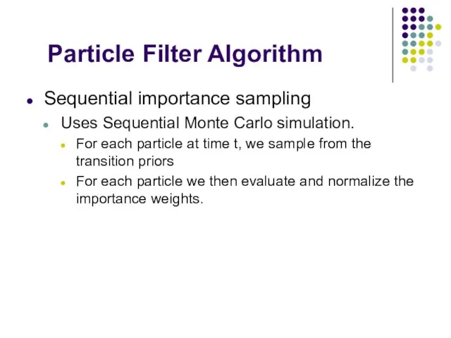
- 17. Particle Filter Algorithm Sequential importance sampling Uses Sequential Monte Carlo simulation. For each particle at time
- 18. Particle Filter Algorithm Selection Step Multiply or discard particles with respect to high or low importance
- 19. Rao-Blackwellised Particle Filter RBPF is an extension on PF. It uses PF to compute the distribution
- 20. RBPF Approach RBPF models the states as Ct is the continuous state representation Dt is the
- 21. Implementation We have implemented the Particle Filter algorithm in Matlab. Our approach towards this project: Reading
- 22. Implementation Color Based Probabilistic Tracking These trackers rely on the deterministic search of a window, whose
- 23. Color Based Probabilistic Tracking The combination of tools used to accomplish a given tracking task depends
- 24. Color Based Probabilistic Tracking Reference Color Window The target object to be tracked forms the reference
- 25. Color Based Probabilistic Tracking State Space We have modeled the states, as its location in each
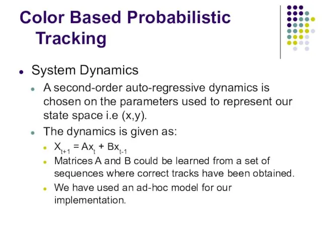
- 26. Color Based Probabilistic Tracking System Dynamics A second-order auto-regressive dynamics is chosen on the parameters used
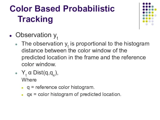
- 27. Color Based Probabilistic Tracking Observation yt The observation yt is proportional to the histogram distance between
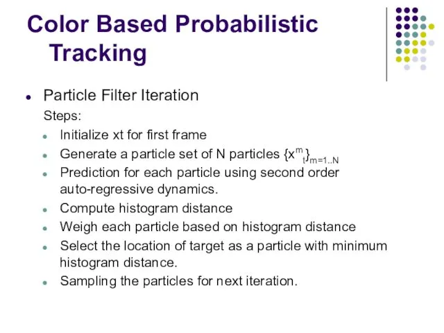
- 28. Color Based Probabilistic Tracking Particle Filter Iteration Steps: Initialize xt for first frame Generate a particle
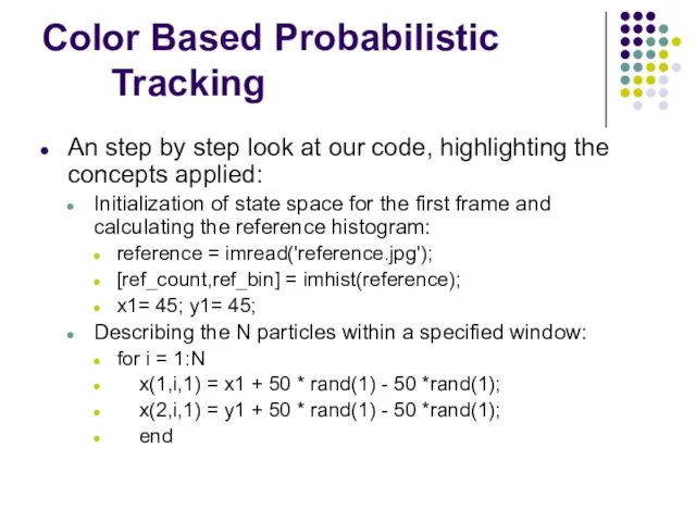
- 29. Color Based Probabilistic Tracking An step by step look at our code, highlighting the concepts applied:
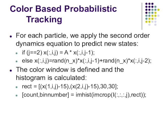
- 30. Color Based Probabilistic Tracking For each particle, we apply the second order dynamics equation to predict
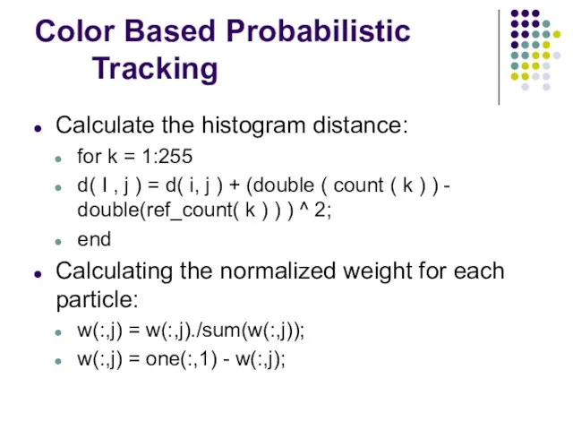
- 31. Color Based Probabilistic Tracking Calculate the histogram distance: for k = 1:255 d( I , j
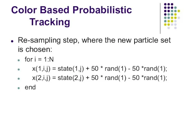
- 32. Color Based Probabilistic Tracking Re-sampling step, where the new particle set is chosen: for i =
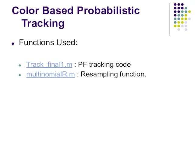
- 33. Color Based Probabilistic Tracking Functions Used: Track_final1.m : PF tracking code multinomialR.m : Resampling function.
- 34. Color Based Probabilistic Tracking: Results
- 35. Applications Video Surveillance Gesture HCI Reality and Visual Effects Medical Imaging State estimation of Rovers in
- 36. Future Work Automatic initialization of reference window. Multi part color window. Multi-object tracking.
- 37. References M. Isard and A. Blake. Condensation–conditional density propagation for visual tracking. Int. J. Computer Vision,
- 39. Скачать презентацию
Overview
Background Information
Basic Particle Filter Theory
Rao Blackwellised Particle Filter
Color Based Probabilistic Tracking
Overview
Background Information
Basic Particle Filter Theory
Rao Blackwellised Particle Filter
Color Based Probabilistic Tracking
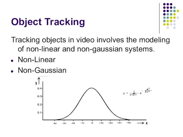
Object Tracking
Tracking objects in video involves the modeling of non-linear and
Object Tracking
Tracking objects in video involves the modeling of non-linear and
Background
In order to model accurately the underlying dynamics of a physical
Background
In order to model accurately the underlying dynamics of a physical
The Particle Filter
Particle Filter is concerned with the problem of
The Particle Filter
Particle Filter is concerned with the problem of
Mathematical Background
Particle Filtering estimates the state of the system, x t,
Mathematical Background
Particle Filtering estimates the state of the system, x t,
Mathematical Background
Particle filtering assumes a Markov Model for system state estimation.
Mathematical Background
Particle filtering assumes a Markov Model for system state estimation.
Mathematical Background
Est(t) = P( x t | y 0 - t
Mathematical Background
Est(t) = P( x t | y 0 - t
Mathematical Background
Final Result:
Est(t) = p(y t | x t ). P(x
Mathematical Background
Final Result:
Est(t) = p(y t | x t ). P(x
Mathematical Background
To implement Particle Filter we need
State Motion model: P(x t
Mathematical Background
To implement Particle Filter we need
State Motion model: P(x t
Mathematical Background
We sample from the proposal and not the posterior for
Mathematical Background
We sample from the proposal and not the posterior for
Basic Particle Filter Theory
A discrete set of samples or particles
Basic Particle Filter Theory
A discrete set of samples or particles
Basic Particle Filter Theory (Cont.)
Particle Filter is concerned with the estimation
Basic Particle Filter Theory (Cont.)
Particle Filter is concerned with the estimation
Basic Particle Filter Theory (Cont.)
System Dynamics ie.Motion Model:
p(x t| x 0:t-1)
Observation
Basic Particle Filter Theory (Cont.)
System Dynamics ie.Motion Model:
p(x t| x 0:t-1)
Observation
Basic Particle Filter Theory (Cont.)
Given N particles (samples) {x(i)0:t-1,z(i)0:t-1}Ni=1 at time
Basic Particle Filter Theory (Cont.)
Given N particles (samples) {x(i)0:t-1,z(i)0:t-1}Ni=1 at time
Basic Particle Filter Theory (Cont.)
The basic Particle Filter algorithm consists of
Basic Particle Filter Theory (Cont.)
The basic Particle Filter algorithm consists of
Particle Filter Algorithm
Sequential importance sampling
Uses Sequential Monte Carlo simulation.
For each
Particle Filter Algorithm
Sequential importance sampling
Uses Sequential Monte Carlo simulation.
For each
Particle Filter Algorithm
Selection Step
Multiply or discard particles with respect to
Particle Filter Algorithm
Selection Step
Multiply or discard particles with respect to
Rao-Blackwellised Particle Filter
RBPF is an extension on PF.
It uses PF to
Rao-Blackwellised Particle Filter
RBPF is an extension on PF.
It uses PF to
RBPF Approach
RBPF models the states as
Ct is the continuous state
RBPF Approach
RBPF models the states as
Ct is the continuous state
Implementation
We have implemented the Particle Filter algorithm in Matlab.
Our approach towards
Implementation
We have implemented the Particle Filter algorithm in Matlab.
Our approach towards
Implementation
Color Based Probabilistic Tracking
These trackers rely on the deterministic search of
Implementation
Color Based Probabilistic Tracking
These trackers rely on the deterministic search of
Color Based Probabilistic Tracking
The combination of tools used to accomplish a
Color Based Probabilistic Tracking
The combination of tools used to accomplish a
Color Based Probabilistic Tracking
Reference Color Window
The target object to be tracked
Color Based Probabilistic Tracking
Reference Color Window
The target object to be tracked
Color Based Probabilistic Tracking
State Space
We have modeled the states, as its
Color Based Probabilistic Tracking
State Space
We have modeled the states, as its
Color Based Probabilistic Tracking
System Dynamics
A second-order auto-regressive dynamics is chosen on
Color Based Probabilistic Tracking
System Dynamics
A second-order auto-regressive dynamics is chosen on
Color Based Probabilistic Tracking
Observation yt
The observation yt is proportional to the
Color Based Probabilistic Tracking
Observation yt
The observation yt is proportional to the
Color Based Probabilistic Tracking
Particle Filter Iteration
Steps:
Initialize xt for first frame
Generate
Color Based Probabilistic Tracking
Particle Filter Iteration
Steps:
Initialize xt for first frame
Generate
Color Based Probabilistic Tracking
An step by step look at our code,
Color Based Probabilistic Tracking
An step by step look at our code,
Color Based Probabilistic Tracking
For each particle, we apply the second order
Color Based Probabilistic Tracking
For each particle, we apply the second order
Color Based Probabilistic Tracking
Calculate the histogram distance:
for k = 1:255
d( I
Color Based Probabilistic Tracking
Calculate the histogram distance:
for k = 1:255
d( I
Color Based Probabilistic Tracking
Re-sampling step, where the new particle set is
Color Based Probabilistic Tracking
Re-sampling step, where the new particle set is
Color Based Probabilistic Tracking
Functions Used:
Track_final1.m : PF tracking code
multinomialR.m : Resampling
Color Based Probabilistic Tracking
Functions Used:
Track_final1.m : PF tracking code
multinomialR.m : Resampling
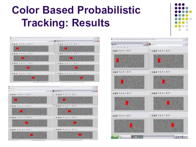
Color Based Probabilistic Tracking: Results
Color Based Probabilistic Tracking: Results
Applications
Video Surveillance
Gesture HCI
Reality and Visual Effects
Medical Imaging
State estimation of
Applications
Video Surveillance
Gesture HCI
Reality and Visual Effects
Medical Imaging
State estimation of
Future Work
Automatic initialization of reference window.
Multi part color window.
Multi-object tracking.
Future Work
Automatic initialization of reference window.
Multi part color window.
Multi-object tracking.
References
M. Isard and A. Blake. Condensation–conditional density propagation for visual tracking.
References
M. Isard and A. Blake. Condensation–conditional density propagation for visual tracking.
 Число и цифра 4
 Подобные слагаемые
 Функции. Пределы функций. Основные понятия теории пределов
 Геометрические построения. Задача на построения с помощью циркуля и линейки
 Решение задач при помощи схематических рисунков (1-2 класс)
 Formālas valodas. Neregulāras valodas
 Путешествие на планету математика
 Четные и нечетные числа
 Вычисление площади с помощью итеграла
 Математическая грамотность
 Классическое определение вероятности
 Развивающая игра по математике
 Смысл действия деления
 Теорема Пифагора
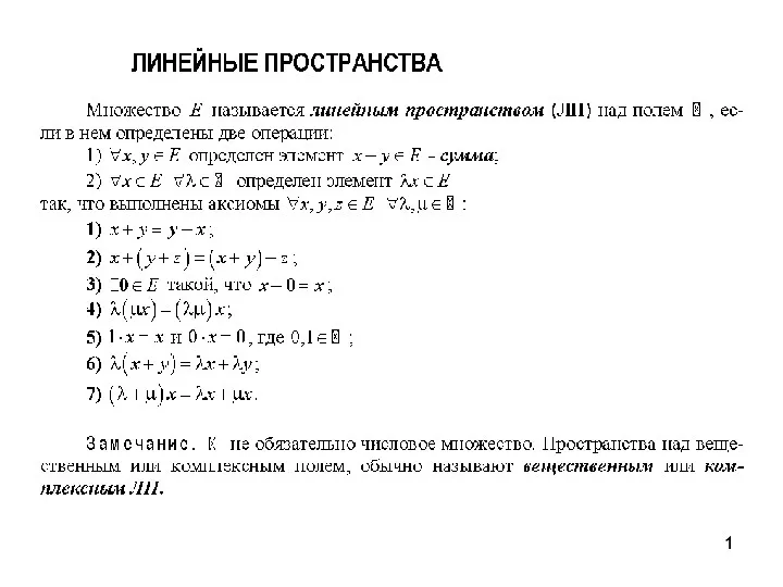 Линейные пространства. Нормированные пространства. Подпространства
 Метод гомогенизации, вариационный подход. (Лекция 12)
 Симметрия. Урок математики для учащихся 4 класса
 Устный счёт
 Сложение рациональных чисел
 Имитационное моделирование. Методология моделирования систем
 Понятие и свойства логарифма
 Показательные и иррациональные уравнения
 Химико – математические проценты
 Медианы, биссектрисы и высоты треугольника
 Теория вероятностей. Предмет теории вероятностей
 Сумма углов треугольника
 Презентация к уроку математики в 3 классе по теме Закрепление. Решение задач.
 Урок математики в 4-ом классе (УМК Гармония). Деление с остатком .