- Value at Risk

Содержание
- 2. The Question Being Asked in VaR “What loss level is such that we are X% confident
- 3. VaR and Regulatory Capital (Business Snapshot 18.1, page 436) Regulators base the capital they require banks
- 4. VaR vs. C-VaR (See Figures 18.1 and 18.2) VaR is the loss level that will not
- 5. Advantages of VaR It captures an important aspect of risk in a single number It is
- 6. Time Horizon Instead of calculating the 10-day, 99% VaR directly analysts usually calculate a 1-day 99%
- 7. Historical Simulation (See Tables 18.1 and 18.2, page 438-439)) Create a database of the daily movements
- 8. Historical Simulation continued Suppose we use m days of historical data Let vi be the value
- 9. The Model-Building Approach The main alternative to historical simulation is to make assumptions about the probability
- 10. Daily Volatilities In option pricing we measure volatility “per year” In VaR calculations we measure volatility
- 11. Daily Volatility continued Strictly speaking we should define σday as the standard deviation of the continuously
- 12. Microsoft Example (page 440) We have a position worth $10 million in Microsoft shares The volatility
- 13. Microsoft Example continued The standard deviation of the change in the portfolio in 1 day is
- 14. Microsoft Example continued We assume that the expected change in the value of the portfolio is
- 15. AT&T Example (page 441) Consider a position of $5 million in AT&T The daily volatility of
- 16. Portfolio Now consider a portfolio consisting of both Microsoft and AT&T Suppose that the correlation between
- 17. S.D. of Portfolio A standard result in statistics states that In this case σX = 200,000
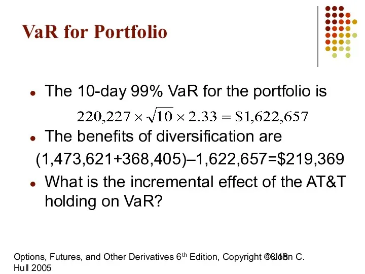
- 18. Options, Futures, and Other Derivatives 6th Edition, Copyright © John C. Hull 2005 18. VaR for
- 19. Value at Risk
- 20. Overview Concepts Components Calculations Corporate perspective Comments
- 21. I VALUE AT RISK - CONCEPTS
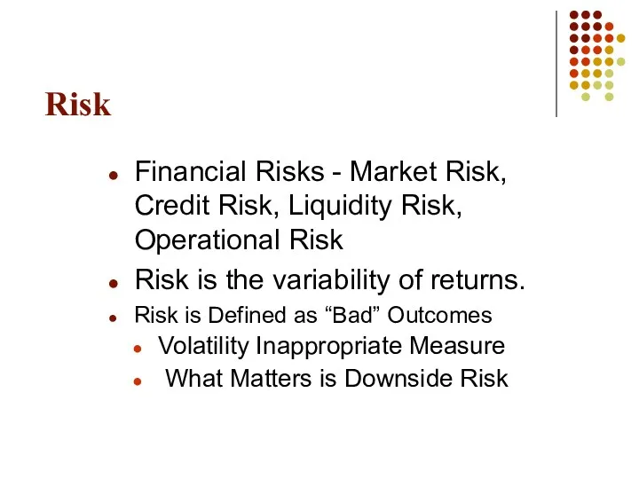
- 22. Risk Financial Risks - Market Risk, Credit Risk, Liquidity Risk, Operational Risk Risk is the variability
- 23. VAR measures Market risk Credit risk of late
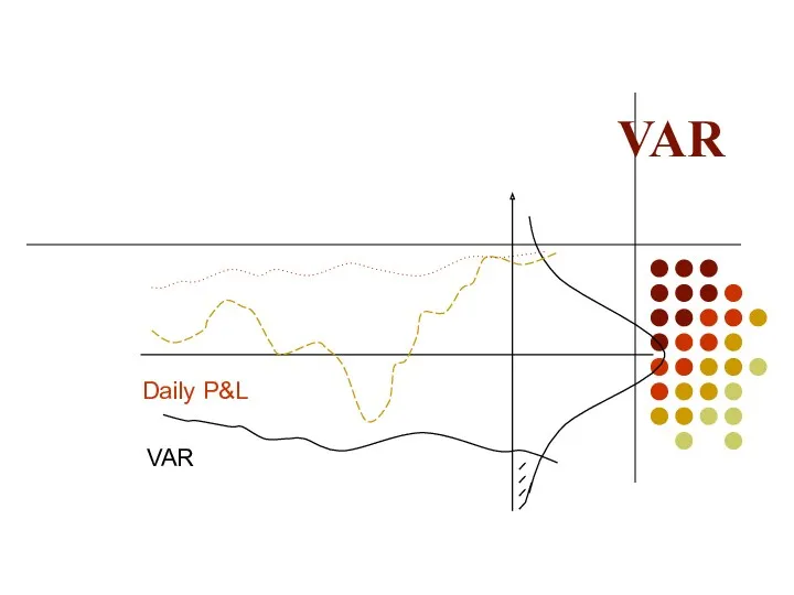
- 24. VAR is an estimate of the adverse impact on P&L in a conservative scenario. It is
- 25. Ingredients - Exposure to market variable Sensitivity Probability of adverse market movement Probability distribution of market
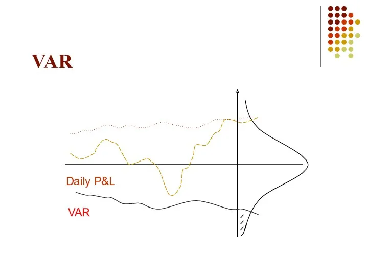
- 26. VAR Daily P&L VAR
- 27. VAR Daily P&L VAR
- 28. II VALUE AT RISK - COMPONENTS
- 29. Key components of VAR Market Factors (MF) Factor Sensitivity (FS) Defeasance Period (DP) Volatility
- 30. Market Factors (MF) A market variable that causes the price of an instrument to change A
- 31. Factor Sensitivity (FS) FS is the change in the value of a position due to a
- 32. Factor Sensitivity - Zero Coupon Bond What is the 1 BP FS of a $2,100 1-year
- 33. Market Volatility Volatility is a measure of the dispersion of a market variable against its mean
- 34. Estimating Volatility 1. Historical data analysis 2. Judgmental 3. Implied (from options prices)
- 35. Defeasance period This is defined as the time elapsed (normally expressed in days) before a position
- 36. Defeasance Factor (DF) DF is the total volatility over the defeasance period On the assumption that
- 37. VAR formula VAR = zα σp √Δt * FS Where: zα is the constant giving the
- 38. VAR Daily P&L VAR
- 39. III VALUE AT RISK - CALCULATIONS
- 40. Sample VAR Calculations Let us consider the following positions: Long EUR against the USD : $
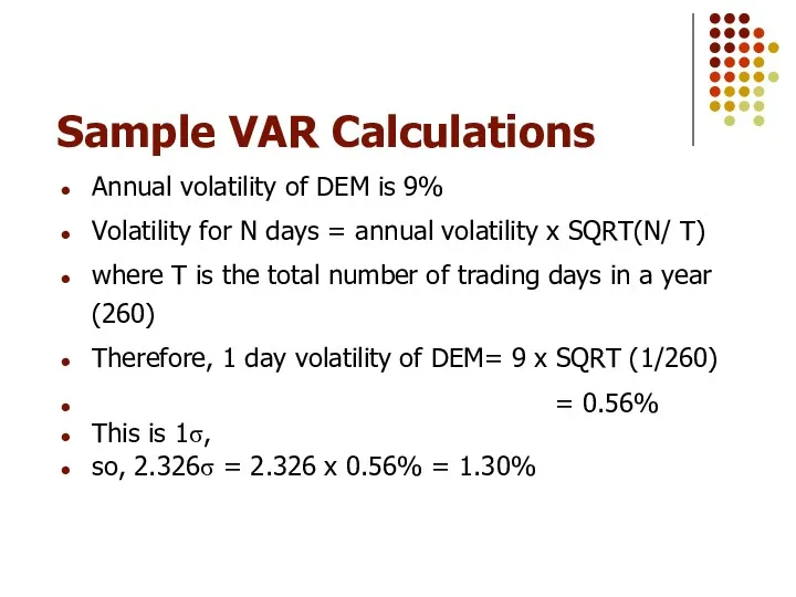
- 41. Sample VAR Calculations Annual volatility of DEM is 9% Volatility for N days = annual volatility
- 42. Sample VAR Calculations Now, a 1% change has an impact of 10,000 (FS) So, a 1.30%
- 43. Sample VAR Calculations Similarly, for JPY, the annual volatility is 12% The 1 day volatility =
- 44. IV VALUE AT RISK FOR CORPORATIONS
- 45. VAR FOR CORPORATIONS Trading portfolios Longer time horizons for close outs Business risk as opposed to
- 46. VAR FOR CORPORATIONS Identify market variables impacting business Map income sensitivity to market variables - Scenario
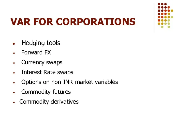
- 47. VAR FOR CORPORATIONS Hedging tools Forward FX Currency swaps Interest Rate swaps Options on non-INR market
- 48. V VALUE AT RISK- A FEW COMMENTS
- 49. Significance of VAR Applicable mainly to trading portfolios Regulatory capital requirements Provides senior executives with a
- 50. VAR : A Few Comments VAR does not represent the maximum loss VAR does not represent
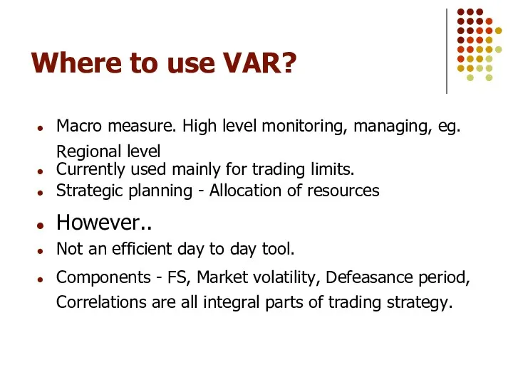
- 51. Where to use VAR? Macro measure. High level monitoring, managing, eg. Regional level Currently used mainly
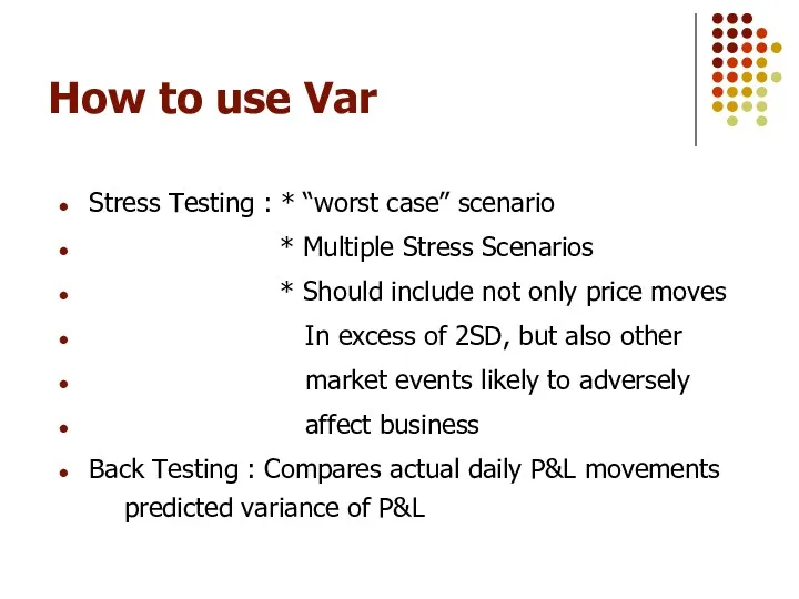
- 52. How to use Var Stress Testing : * “worst case” scenario * Multiple Stress Scenarios *
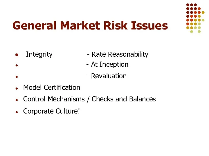
- 53. General Market Risk Issues Integrity - Rate Reasonability - At Inception - Revaluation Model Certification Control
- 55. Скачать презентацию

The Question Being Asked in VaR
“What loss level is such that
The Question Being Asked in VaR
“What loss level is such that
VaR and Regulatory Capital
(Business Snapshot 18.1, page 436)
Regulators base the capital
VaR and Regulatory Capital
(Business Snapshot 18.1, page 436)
Regulators base the capital
VaR vs. C-VaR
(See Figures 18.1 and 18.2)
VaR is the loss
VaR vs. C-VaR
(See Figures 18.1 and 18.2)
VaR is the loss
Advantages of VaR
It captures an important aspect of risk
in a single
Advantages of VaR
It captures an important aspect of risk
in a single
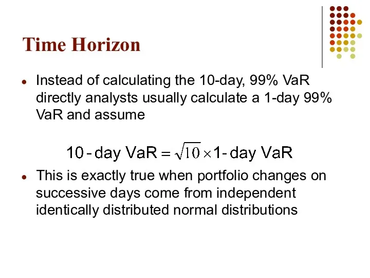
Time Horizon
Instead of calculating the 10-day, 99% VaR directly analysts usually
Time Horizon
Instead of calculating the 10-day, 99% VaR directly analysts usually
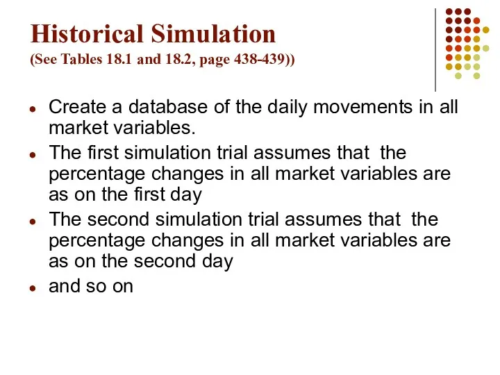
Historical Simulation
(See Tables 18.1 and 18.2, page 438-439))
Create a database
Historical Simulation
(See Tables 18.1 and 18.2, page 438-439))
Create a database
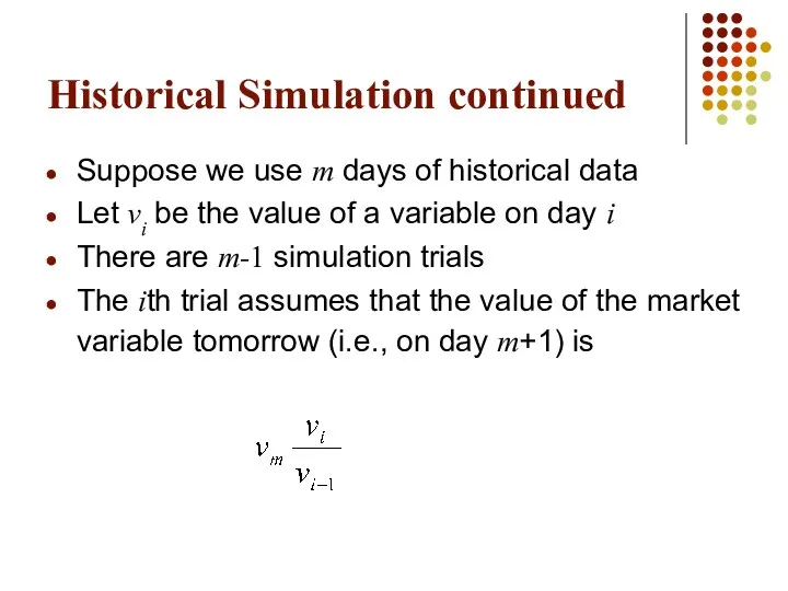
Historical Simulation continued
Suppose we use m days of historical data
Let vi
Historical Simulation continued
Suppose we use m days of historical data
Let vi
The Model-Building Approach
The main alternative to historical simulation is to make
The Model-Building Approach
The main alternative to historical simulation is to make
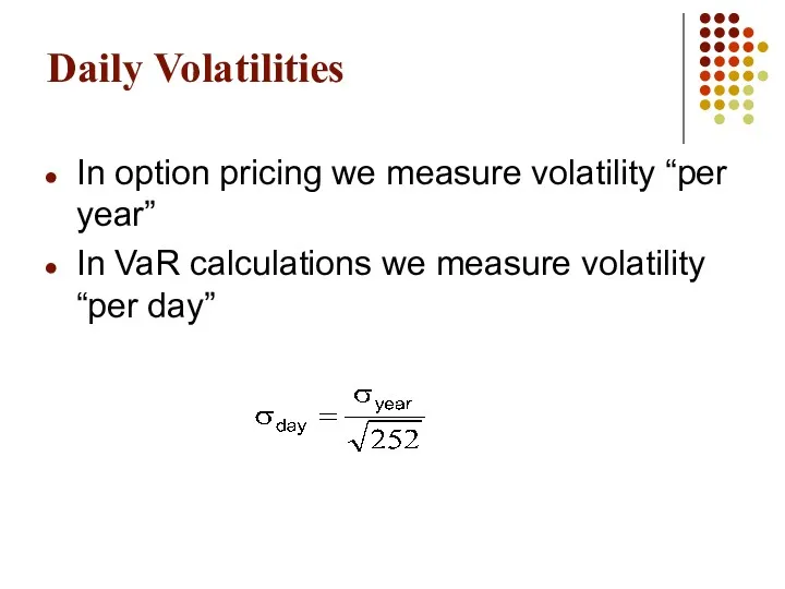
Daily Volatilities
In option pricing we measure volatility “per year”
In VaR calculations
Daily Volatilities
In option pricing we measure volatility “per year”
In VaR calculations
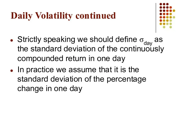
Daily Volatility continued
Strictly speaking we should define σday as the standard
Daily Volatility continued
Strictly speaking we should define σday as the standard
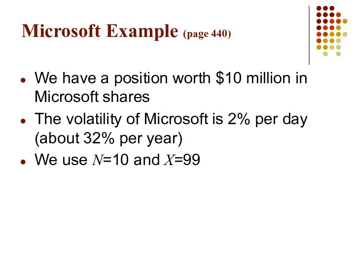
Microsoft Example (page 440)
We have a position worth $10 million in
Microsoft Example (page 440)
We have a position worth $10 million in
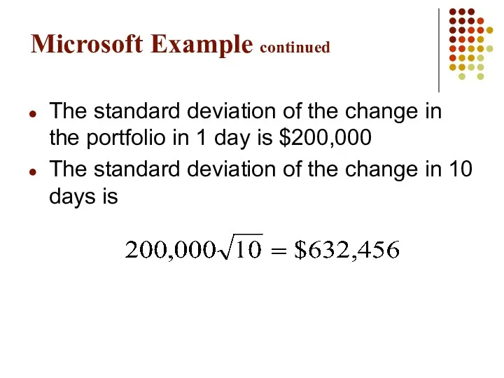
Microsoft Example continued
The standard deviation of the change in the portfolio
Microsoft Example continued
The standard deviation of the change in the portfolio
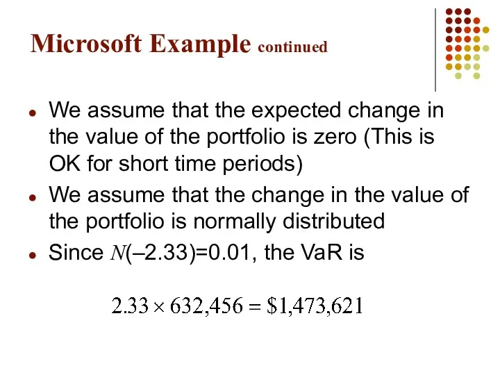
Microsoft Example continued
We assume that the expected change in the value
Microsoft Example continued
We assume that the expected change in the value
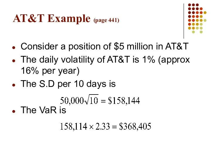
AT&T Example (page 441)
Consider a position of $5 million in AT&T
The
AT&T Example (page 441)
Consider a position of $5 million in AT&T
The
Portfolio
Now consider a portfolio consisting of both Microsoft and AT&T
Suppose that
Portfolio
Now consider a portfolio consisting of both Microsoft and AT&T
Suppose that
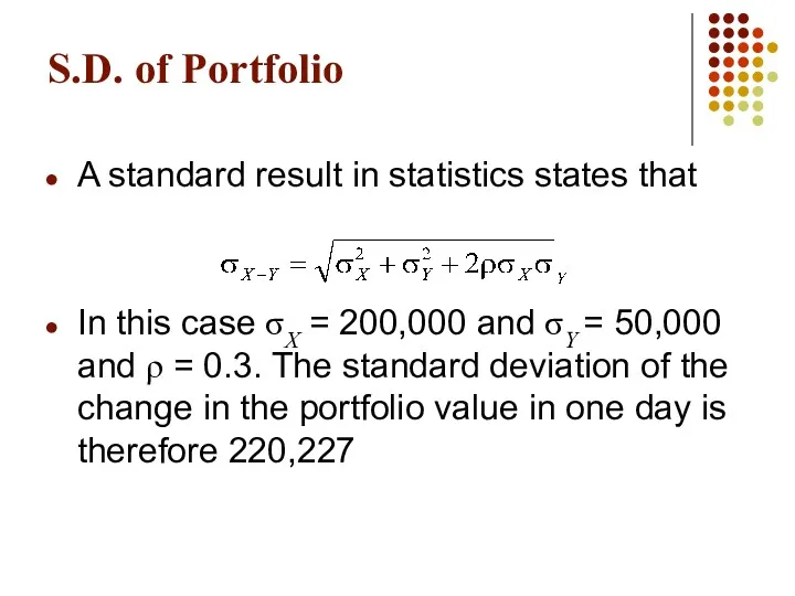
S.D. of Portfolio
A standard result in statistics states that
In this case
S.D. of Portfolio
A standard result in statistics states that
In this case
Options, Futures, and Other Derivatives 6th Edition, Copyright © John C.
Options, Futures, and Other Derivatives 6th Edition, Copyright © John C.

Value at Risk
Value at Risk

Overview
Concepts
Components
Calculations
Corporate perspective
Comments
Overview
Concepts
Components
Calculations
Corporate perspective
Comments
I VALUE AT RISK - CONCEPTS
I VALUE AT RISK - CONCEPTS
Risk
Financial Risks - Market Risk, Credit Risk, Liquidity Risk, Operational Risk
Risk
Risk
Financial Risks - Market Risk, Credit Risk, Liquidity Risk, Operational Risk
Risk
VAR measures
Market risk
Credit risk of late
VAR measures
Market risk
Credit risk of late
VAR is an estimate of the adverse impact on P&L in
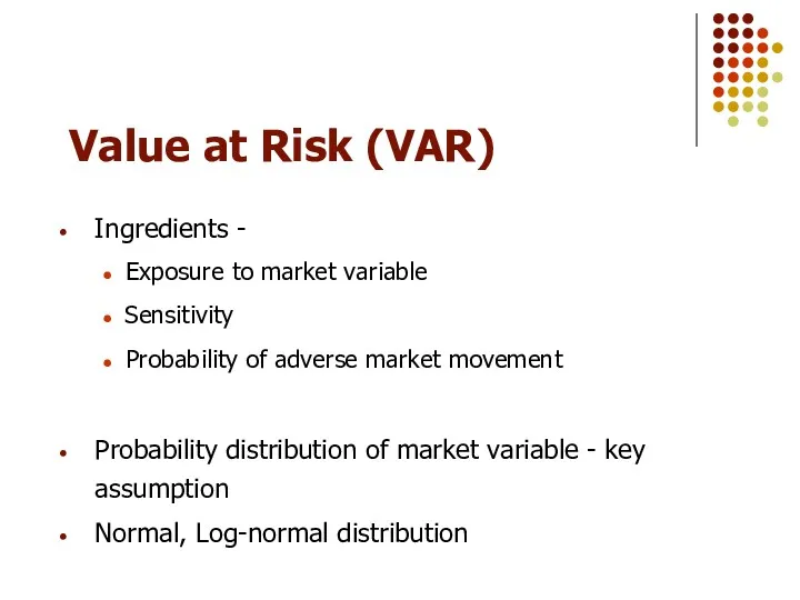
Ingredients -
Exposure to market variable
Sensitivity
Probability of adverse
Exposure to market variable
Sensitivity
Probability of adverse

VAR
Daily P&L
VAR
VAR
Daily P&L
VAR
VAR
Daily P&L
VAR
VAR
Daily P&L
VAR
II VALUE AT RISK - COMPONENTS
II VALUE AT RISK - COMPONENTS
Key components of VAR
Market Factors (MF)
Factor Sensitivity (FS)
Defeasance Period (DP)
Volatility
Key components of VAR
Market Factors (MF)
Factor Sensitivity (FS)
Defeasance Period (DP)
Volatility
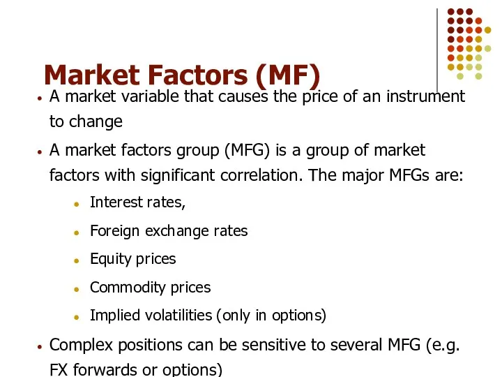
Market Factors (MF)
A market variable that causes the price of an
Market Factors (MF)
A market variable that causes the price of an
Factor Sensitivity (FS)
FS is the change in the value of a
Factor Sensitivity (FS)
FS is the change in the value of a
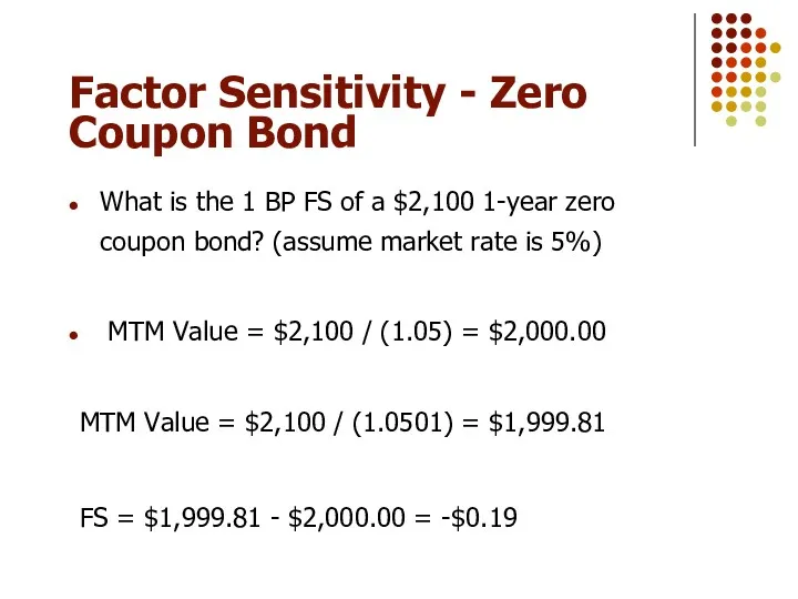
Factor Sensitivity - Zero Coupon Bond
What is the 1 BP FS
Factor Sensitivity - Zero Coupon Bond
What is the 1 BP FS
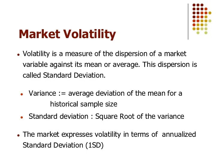
Market Volatility
Volatility is a measure of the dispersion of a market
Market Volatility
Volatility is a measure of the dispersion of a market
Estimating Volatility
1. Historical data analysis
2. Judgmental
3. Implied (from options
Estimating Volatility
1. Historical data analysis
2. Judgmental
3. Implied (from options
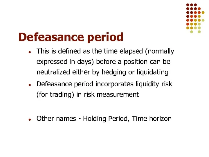
Defeasance period
This is defined as the time elapsed (normally expressed in
Defeasance period
This is defined as the time elapsed (normally expressed in
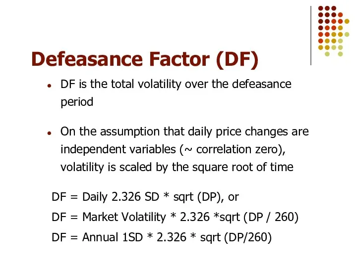
Defeasance Factor (DF)
DF is the total volatility over the defeasance period
On
Defeasance Factor (DF)
DF is the total volatility over the defeasance period
On
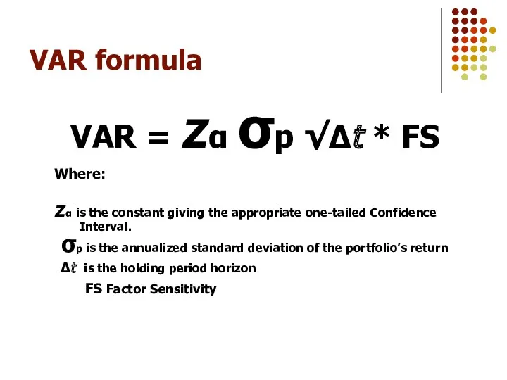
VAR formula
VAR = zα σp √Δt * FS
Where:
zα is the constant
VAR formula
VAR = zα σp √Δt * FS
Where:
zα is the constant
VAR
Daily P&L
VAR
VAR
Daily P&L
VAR
III VALUE AT RISK - CALCULATIONS
III VALUE AT RISK - CALCULATIONS
Sample VAR Calculations
Let us consider the following positions:
Long EUR against the
Sample VAR Calculations
Let us consider the following positions:
Long EUR against the
Sample VAR Calculations
Annual volatility of DEM is 9%
Volatility for N days
Sample VAR Calculations
Annual volatility of DEM is 9%
Volatility for N days
Sample VAR Calculations
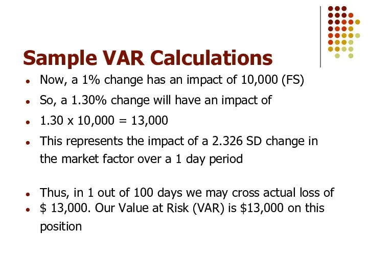
Now, a 1% change has an impact of 10,000
Sample VAR Calculations
Now, a 1% change has an impact of 10,000
Sample VAR Calculations
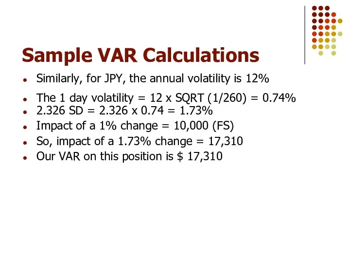
Similarly, for JPY, the annual volatility is 12%
The 1
Sample VAR Calculations
Similarly, for JPY, the annual volatility is 12%
The 1

IV VALUE AT RISK FOR CORPORATIONS
IV VALUE AT RISK FOR CORPORATIONS
VAR FOR CORPORATIONS
Trading portfolios
Longer time horizons for close outs
VAR FOR CORPORATIONS
Trading portfolios
Longer time horizons for close outs
VAR FOR CORPORATIONS
Identify market variables impacting business
Map income
VAR FOR CORPORATIONS
Identify market variables impacting business
Map income
VAR FOR CORPORATIONS
Hedging tools
Forward FX
Currency swaps
Interest
VAR FOR CORPORATIONS
Hedging tools
Forward FX
Currency swaps
Interest
V VALUE AT RISK- A FEW COMMENTS
V VALUE AT RISK- A FEW COMMENTS
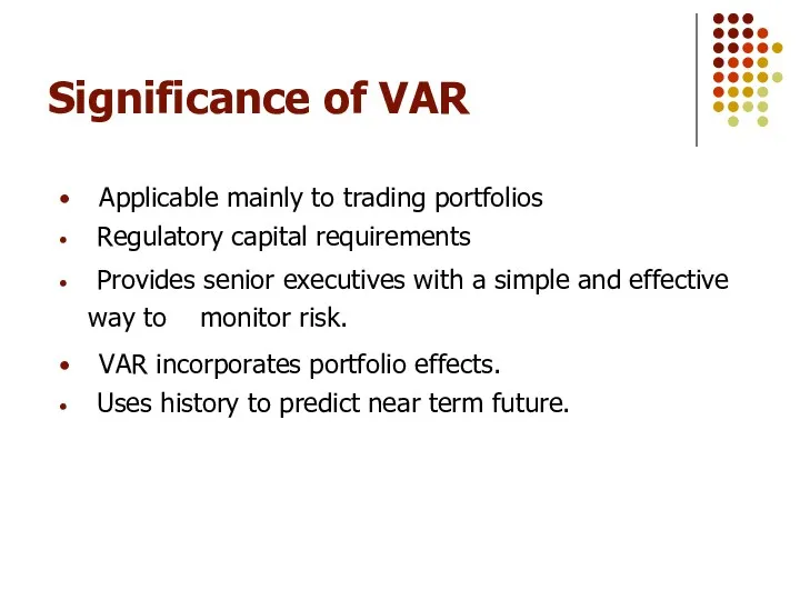
Significance of VAR
Applicable mainly to trading portfolios
Regulatory capital requirements
Significance of VAR
Applicable mainly to trading portfolios
Regulatory capital requirements
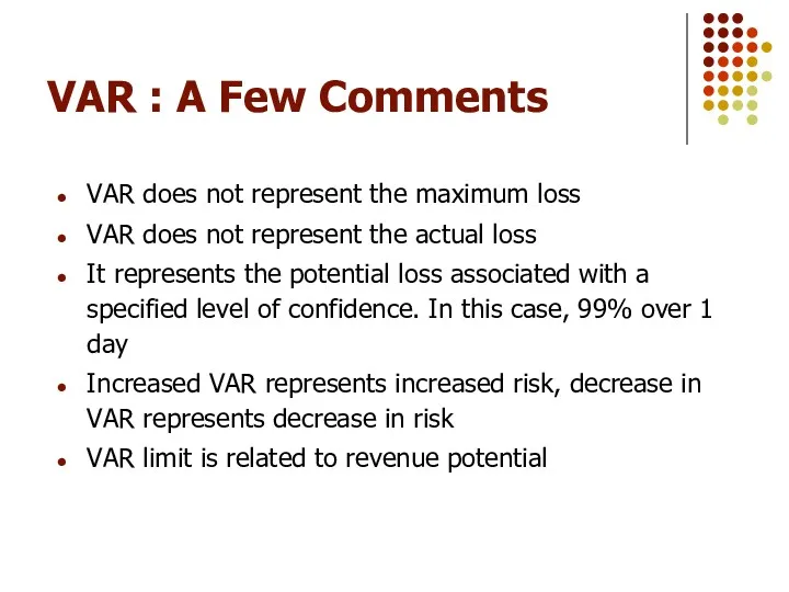
VAR : A Few Comments
VAR does not represent the maximum loss
VAR
VAR : A Few Comments
VAR does not represent the maximum loss
VAR
Where to use VAR?
Macro measure. High level monitoring, managing, eg. Regional
Where to use VAR?
Macro measure. High level monitoring, managing, eg. Regional
How to use Var
Stress Testing : * “worst case” scenario
*
How to use Var
Stress Testing : * “worst case” scenario
*
General Market Risk Issues
Integrity - Rate Reasonability
- At Inception
General Market Risk Issues
Integrity - Rate Reasonability
- At Inception
 Семейный бюджет
 Финансы. Задачи. Тема 1
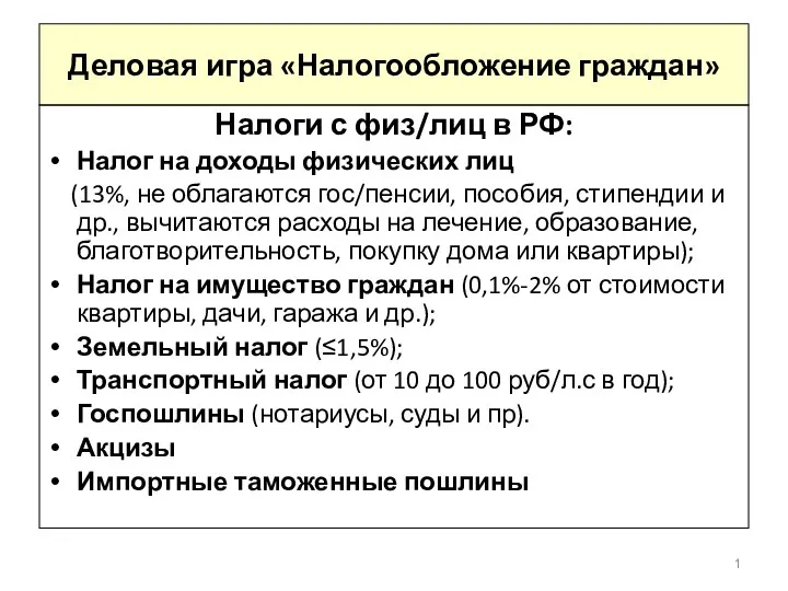 Деловая игра Налогообложение граждан
 Ең төменгі жалақы және кедейлер
 Деньги и их функции
 Учет сырья, продуктов и тары в кладовых п о п
 Внешнеторговые документарные операции (2)
 Инвестиции и методы финансирования
 Центральный банк и его роль в банковской системе
 Перевод работников АО Красная звезда на новые условия оплаты труда
 Муниципальное образование город Алапаевск. Бюджет для граждан
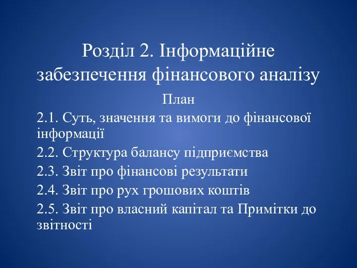 Інформаційне забезпечення фінансового аналізу. Лекція 2
 Страховой рынок и его структура
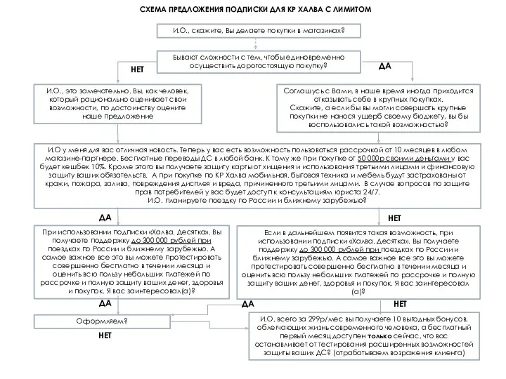 Схема предложения подписки Халва. Десятка
 Учет в бюджетных учреждениях
 Бюджетирование проектов. (Лекция 7)
 Составление смет на пусконаладочные работы
 Оценка целостных имущественных комплексов
 Бухгалтерлік есеп нысандары
 Виды кредитов
 Портфель финансовых активов
 Денежный оборот и его структура
 Налоговая и бухгалтерская отчетность садоводческих товариществ
 Бухгалтерский Учет кредитов и займов
 Выручка. Международные стандарты финансовой отчётности (МСФО 18)
 Страховой надзор
 Международные ценные бумаги. Эффективная система внешних заимствований. Тема 5
 Фінансові інвестиції