- Evolution of Convolutional Neural Networks

Содержание
- 2. Lenet-5 (1998) MNIST: handwritten digits 70,000 28x28 pixel images Gray scale 10 classes CIFAR-10: simple objects
- 3. ImageNet Dataset (2010) 10M hand labelled images Variable resolution (between 512 and 256 pixels) 22k categories
- 4. AlexNet (2012) ReLU Dropout Overlapping Max Pooling No pre-training 8 layers, 60M parameters 90% of weights
- 5. Network in Network (2014) Insert MLP between conv layers: Extra non-linearity (ReLU) Better combination of feature
- 6. VGG (2014) Increase depth and width Use only 3x3 filters 16 layers and lots of parameters
- 7. GoogLeNet (Inception v1, 2014) How to reduce amount of computation? Move from fully connected to sparse
- 8. Batch Normalization (Inception v2) Problem: “Internal Covariate Shift” Updating weights changes distribution of outputs at each
- 9. Inception v3 (2015) Efficient ways to scale up GoogLeNet Gradually reduce dimensionality, but increase number of
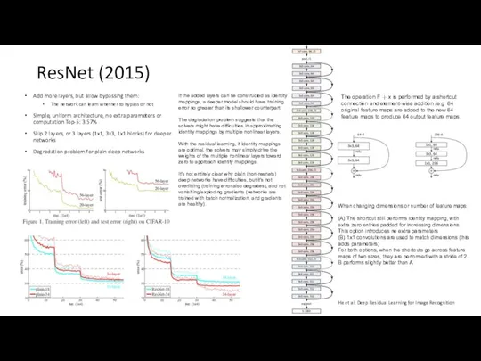
- 10. ResNet (2015) Add more layers, but allow bypassing them: The network can learn whether to bypass
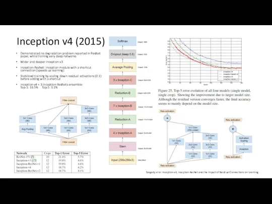
- 11. Inception v4 (2015) Demonstrated no degradation problem reported in ResNet paper, while training very deep networks
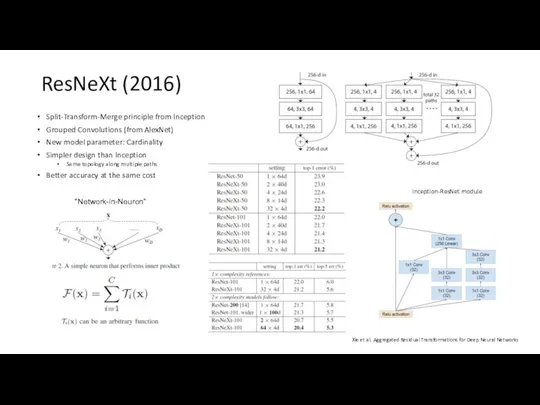
- 12. ResNeXt (2016) Split-Transform-Merge principle from Inception Grouped Convolutions (from AlexNet) New model parameter: Cardinality Simpler design
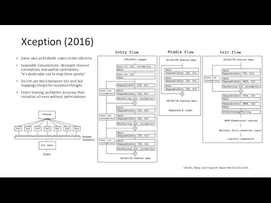
- 13. Xception (2016) Same idea as ResNeXt, taken to the eXtreme Separable Convolutions: decouple channel correlations and
- 14. DenseNet (2016) Feature maps of each layer serve as input to all consecutive layers Feature maps
- 15. What’s next: Dense ResNeXt? Combine grouped convolutions idea from ResNeXt and full connectivity of DenseNet Replace
- 17. Скачать презентацию
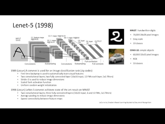
Lenet-5 (1998)
MNIST: handwritten digits
70,000 28x28 pixel images
Gray scale
10 classes
CIFAR-10:
Lenet-5 (1998)
MNIST: handwritten digits
70,000 28x28 pixel images
Gray scale
10 classes
CIFAR-10:
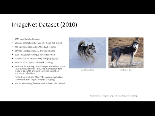
ImageNet Dataset (2010)
10M hand labelled images
Variable resolution (between 512 and 256
ImageNet Dataset (2010)
10M hand labelled images
Variable resolution (between 512 and 256
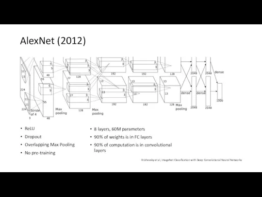
AlexNet (2012)
ReLU
Dropout
Overlapping Max Pooling
No pre-training
8 layers, 60M parameters
90% of weights is
AlexNet (2012)
ReLU
Dropout
Overlapping Max Pooling
No pre-training
8 layers, 60M parameters
90% of weights is
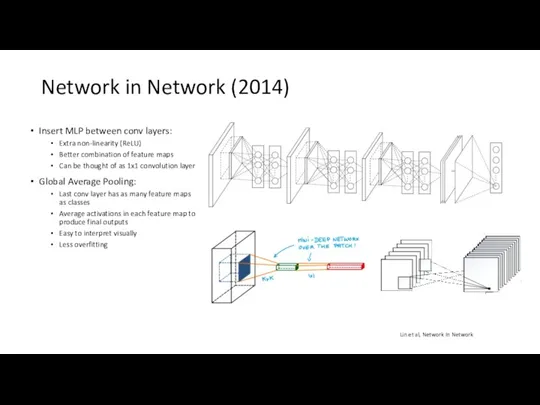
Network in Network (2014)
Insert MLP between conv layers:
Extra non-linearity (ReLU)
Better
Network in Network (2014)
Insert MLP between conv layers:
Extra non-linearity (ReLU)
Better
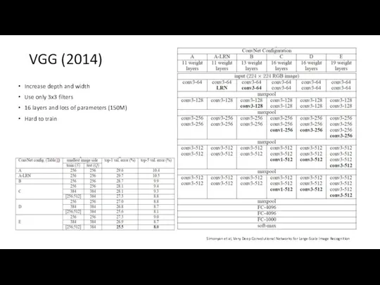
VGG (2014)
Increase depth and width
Use only 3x3 filters
16 layers and lots
VGG (2014)
Increase depth and width
Use only 3x3 filters
16 layers and lots
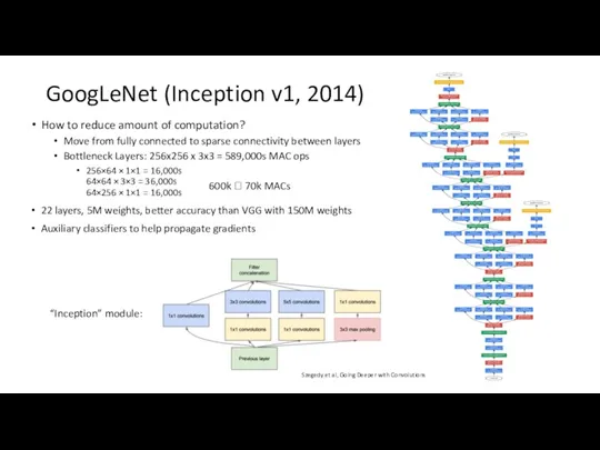
GoogLeNet (Inception v1, 2014)
How to reduce amount of computation?
Move from fully
GoogLeNet (Inception v1, 2014)
How to reduce amount of computation?
Move from fully
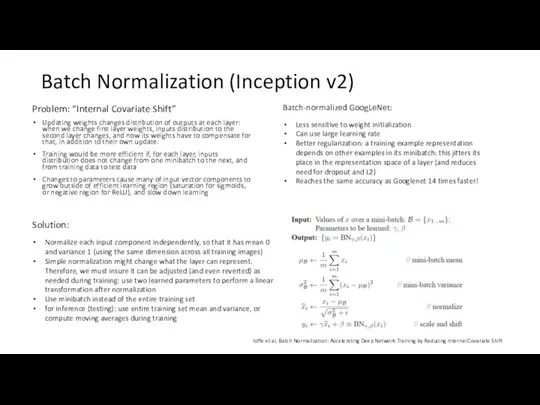
Batch Normalization (Inception v2)
Problem: “Internal Covariate Shift”
Updating weights changes distribution of
Batch Normalization (Inception v2)
Problem: “Internal Covariate Shift”
Updating weights changes distribution of
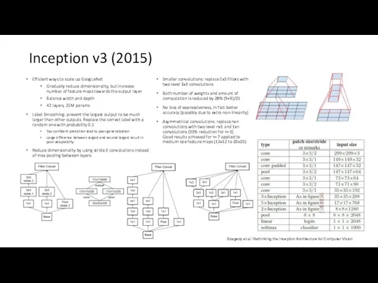
Inception v3 (2015)
Efficient ways to scale up GoogLeNet
Gradually reduce dimensionality, but
Inception v3 (2015)
Efficient ways to scale up GoogLeNet
Gradually reduce dimensionality, but
ResNet (2015)
Add more layers, but allow bypassing them:
The network can learn
ResNet (2015)
Add more layers, but allow bypassing them:
The network can learn
Inception v4 (2015)
Demonstrated no degradation problem reported in ResNet paper, while
Inception v4 (2015)
Demonstrated no degradation problem reported in ResNet paper, while
ResNeXt (2016)
Split-Transform-Merge principle from Inception
Grouped Convolutions (from AlexNet)
New model parameter: Cardinality
ResNeXt (2016)
Split-Transform-Merge principle from Inception
Grouped Convolutions (from AlexNet)
New model parameter: Cardinality
Xception (2016)
Same idea as ResNeXt, taken to the eXtreme
Separable Convolutions: decouple
Xception (2016)
Same idea as ResNeXt, taken to the eXtreme
Separable Convolutions: decouple
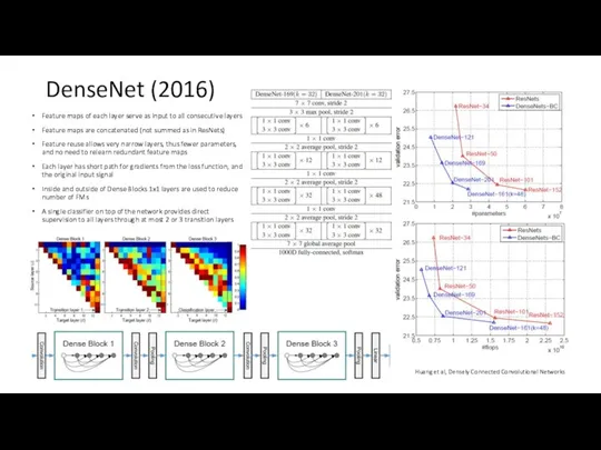
DenseNet (2016)
Feature maps of each layer serve as input to all
DenseNet (2016)
Feature maps of each layer serve as input to all
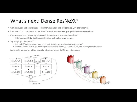
What’s next: Dense ResNeXt?
Combine grouped convolutions idea from ResNeXt and full
What’s next: Dense ResNeXt?
Combine grouped convolutions idea from ResNeXt and full
 Помехоустойчивое кодирование
 Инструкция по работе с функционалом Справочник сотрудников в ИБ Мой Бизнес в части ЗП проектов
 Ғаламтор ғажайыбы
 Программирование на Python. Урок 9. Новая игра и ООП
 11_Позиционирование
 Программное обеспечение робота
 Тестировщик программного обеспечения. Занятие 13. Тестирование web-приложений
 Циклический алгоритм
 Bootstrap. Самые современные технологии CSS и HTML
 Создание электронного портфолио
 Информационные технологии. Информационное обеспечение
 Access List-ы
 Лекция 01_Введение .Типы данных.Мат.операции.Ввод_вывод
 Общая характеристика табличного процессора
 Презентация Клавиши клавиатуры
 Применение методов глубокого обучения к задаче конкурирующей перколяции
 Безпека в Інтернеті. Безпечне зберігання даних
 ВКР: Оптимизация сбора информации, её проверки и анализа для материалов СМИ в журналистской деятельности
 20231001_prezentatsiya
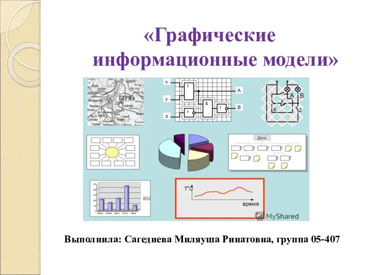 Графические информационные модели
 Особливості програмування під Windows
 Разработка программ управления компьютером
 Тэгтердің атрибуттары. Мәтінді. Безендіру
 Разработка детской настольной игры
 Пошук відомостей у мережі інтернет
 Информационные процессы. Лекция 4
 Открытое занятие Берём интервью
 Интернет вещей. Возможности логистической интеграции, сферы применения, примеры и стоимость реализации