- M/EEG source analysis

Содержание
- 2. Overview Forward Models for M/EEG Variational Bayesian Dipole Estimation (ECD) Empirical Bayesian Distributed Estimation Multimodal integration
- 3. Overview Forward Models for M/EEG Variational Bayesian Dipole Estimation (ECD) Empirical Bayesian Distributed Estimation Multimodal integration
- 4. Likelihood Prior Posterior Evidence Bayesian Perspective Forward Problem Inverse Problem Data Parameters Model
- 5. Likelihood Forward Problem: Physics Kirkoff’s law: Electrical potential Quasi-static Maxwell’s Equations: Orientation Location Current density: (EEG)
- 6. Likelihood Forward Problem: Physics Orientation Location depends on: Can have analytic or numerical form… location (orientation)
- 7. Forward Problem: Head Models Concentric Spheres: Pros: Analytic; Fast to compute Cons: Head not spherical; Conductivity
- 8. Forward Problem: Meshes 3 important surfaces for BEMs are those with large changes in conductivity: Scalp
- 9. Forward Problem: Canonical Meshes Rather than extract surfaces from individuals MRIs, why not warp Template surfaces
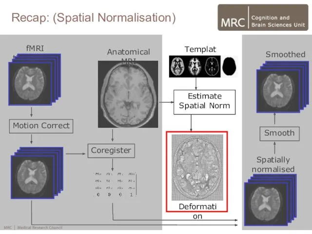
- 10. fMRI time-series Motion Correct Anatomical MRI Coregister Deformation Estimate Spatial Norm Spatially normalised Smooth Smoothed Template
- 11. Forward Problem: Canonical Meshes Rather than extract surfaces from individuals MRIs, why not warp Template surfaces
- 12. Likelihood Forward Problem: ECD vs Distributed Orientation Location For small number of Equivalent Current Dipoles (ECD)
- 13. Overview Forward Models for M/EEG Variational Bayesian Dipole Estimation (ECD) Empirical Bayesian Distributed Estimation Multimodal integration
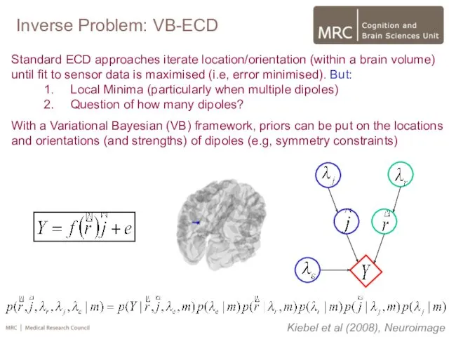
- 14. Inverse Problem: VB-ECD Standard ECD approaches iterate location/orientation (within a brain volume) until fit to sensor
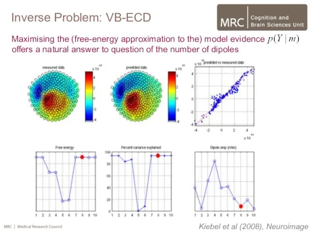
- 15. Inverse Problem: VB-ECD Maximising the (free-energy approximation to the) model evidence offers a natural answer to
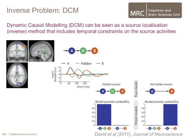
- 16. Inverse Problem: DCM Dynamic Causal Modelling (DCM) can be seen as a source localisation (inverse) method
- 17. Overview Forward Models for M/EEG Variational Bayesian Dipole Estimation (ECD) Empirical Bayesian Distributed Estimation Multimodal integration
- 18. Y = Data n sensors J = Sources p>>n sources L = Leadfields n sensors x
- 19. Phillips et al (2002), Neuroimage Inverse Problem: Standard L2-norm “Minimum Norm” “Loreta” (D=Laplacian) “Depth-Weighted” “Beamformer” “Tikhonov
- 20. Phillips et al (2005), Neuroimage Likelihood: C(e) = n x n Sensor (error) covariance Prior: C(j)
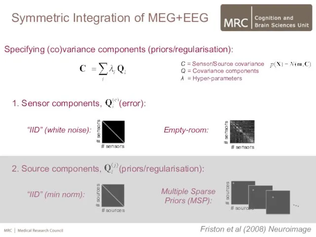
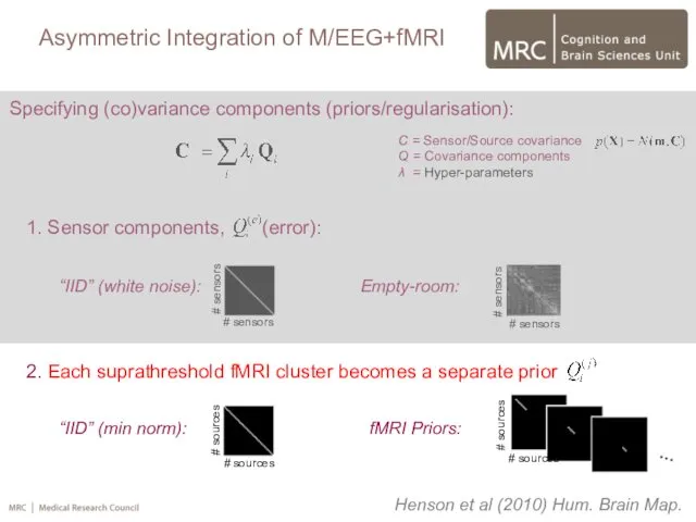
- 21. Specifying (co)variance components (priors/regularisation): 1. Sensor components, (error): C = Sensor/Source covariance Q = Covariance components
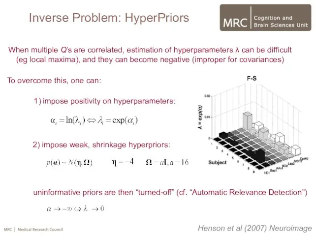
- 22. Henson et al (2007) Neuroimage When multiple Q’s are correlated, estimation of hyperparameters λ can be
- 23. Henson et al (2007) Neuroimage When multiple Q’s are correlated, estimation of hyperparameters λ can be
- 24. Friston et al (2008) Neuroimage Fixed Variable Data Source and sensor space Inverse Problem: Full (DAG)
- 25. Friston et al (2002) Neuroimage 1. Obtain Restricted Maximum Likelihood (ReML) estimates of the hyperparameters (λ)
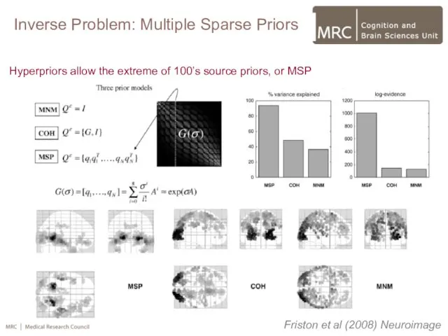
- 26. Hyperpriors allow the extreme of 100’s source priors, or MSP Inverse Problem: Multiple Sparse Priors …
- 27. Hyperpriors allow the extreme of 100’s source priors, or MSP Inverse Problem: Multiple Sparse Priors Friston
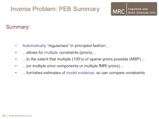
- 28. Summary: Automatically “regularises” in principled fashion… …allows for multiple constraints (priors)… …to the extent that multiple
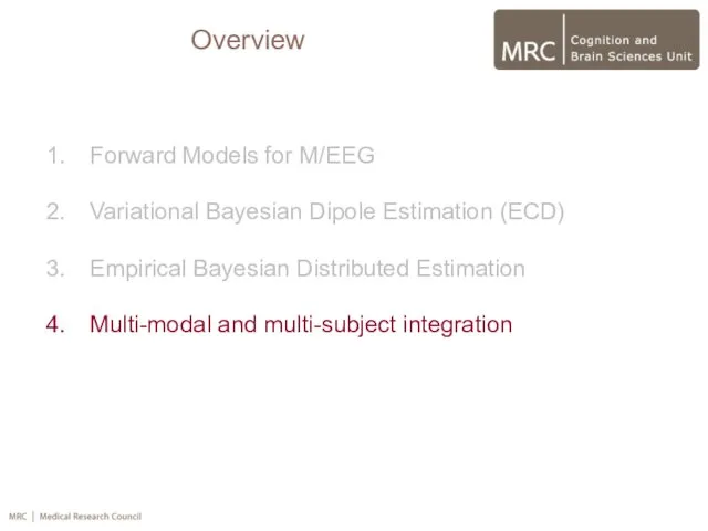
- 29. Overview Forward Models for M/EEG Variational Bayesian Dipole Estimation (ECD) Empirical Bayesian Distributed Estimation Multi-modal and
- 30. Multi-subject Integration (Group Inversion) Specifying (co)variance components (priors/regularisation): 1. Sensor components, (error): C = Sensor/Source covariance
- 31. Specifying (co)variance components (priors/regularisation): 1. Sensor components, (error): C = Sensor/Source covariance Q = Covariance components
- 32. Litvak & Friston (2008) Neuroimage Fixed Variable Data Source and sensor space Multi-subject Integration (as before)
- 33. Litvak & Friston (2008) Neuroimage Fixed Variable Data Source and sensor space Multi-subject Integration
- 34. Concatenate data across subjects Common source-level priors: Subject-specific sensor-level priors: Litvak & Friston (2008) Neuroimage …having
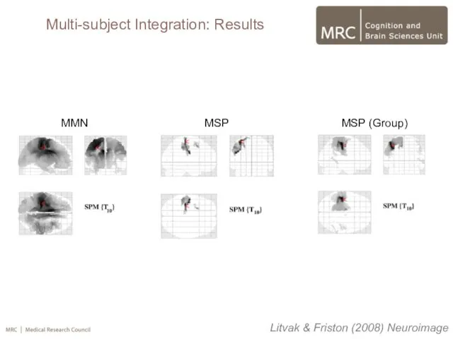
- 35. Litvak & Friston (2008) Neuroimage MMN MSP MSP (Group) Multi-subject Integration: Results
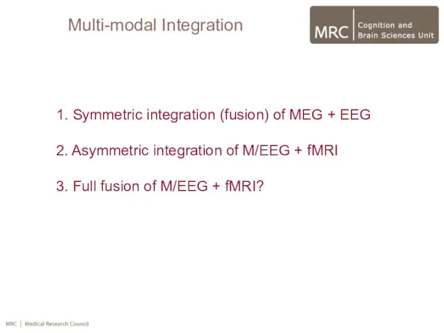
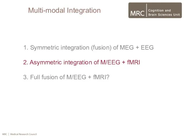
- 36. Multi-modal Integration 1. Symmetric integration (fusion) of MEG + EEG 2. Asymmetric integration of M/EEG +
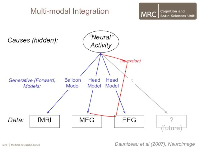
- 37. fMRI MEG ? (future) Data: Causes (hidden): Generative (Forward) Models: Balloon Model Head Model ? EEG
- 38. Asymmetric Integration fMRI MEG ? (future) Data: Causes (hidden): Generative (Forward) Models: Balloon Model Head Model
- 39. Multi-modal Integration 1. Symmetric integration (fusion) of MEG + EEG 2. Asymmetric integration of M/EEG +
- 40. Specifying (co)variance components (priors/regularisation): 1. Sensor components, (error): C = Sensor/Source covariance Q = Covariance components
- 41. Specifying (co)variance components (priors/regularisation): 1. Sensor components, (error): Ci(e) = Sensor error covariance for ith modality
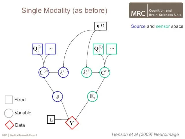
- 42. Henson et al (2009) Neuroimage Fixed Variable Data Source and sensor space Single Modality (as before)
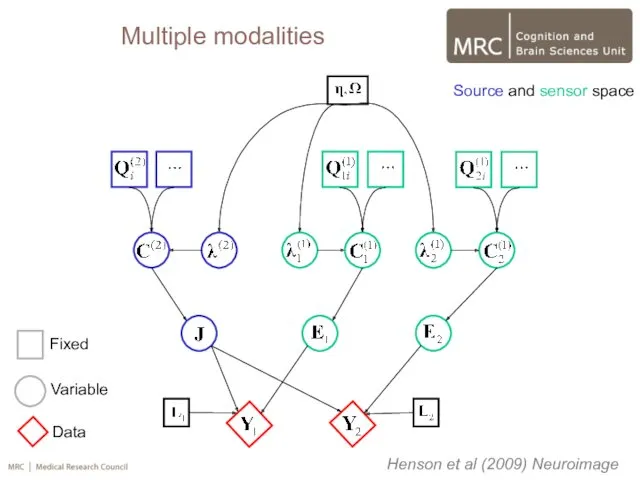
- 43. Henson et al (2009) Neuroimage Fixed Variable Data Source and sensor space Multiple modalities
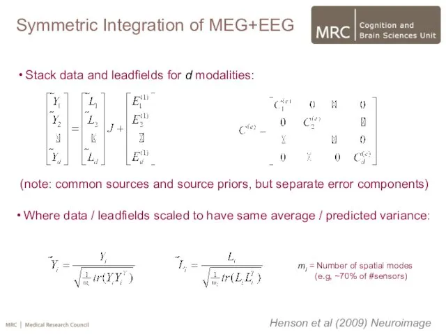
- 44. Henson et al (2009) Neuroimage Stack data and leadfields for d modalities: Where data / leadfields
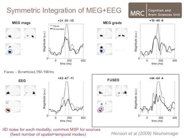
- 45. ERs from 12 subjects for 3 simultaneously-acquired Neuromag sensor-types: RMS fT/m μV Faces Scrambled fT Magnetometers
- 46. MEG mags MEG grads EEG FUSED +31 -51 -15 +19 -48 -6 +43 -67 -11 +44
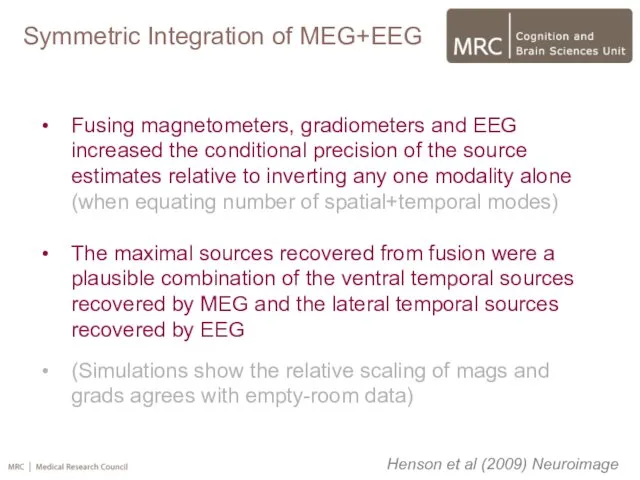
- 47. Henson et al (2009) Neuroimage Fusing magnetometers, gradiometers and EEG increased the conditional precision of the
- 48. Multi-modal Integration 1. Symmetric integration (fusion) of MEG + EEG 2. Asymmetric integration of M/EEG +
- 49. Asymmetric Integration of M/EEG+fMRI Specifying (co)variance components (priors/regularisation): 1. Sensor components, (error): C = Sensor/Source covariance
- 50. Henson et al (2010) Hum. Brain Map. Specifying (co)variance components (priors/regularisation): 1. Sensor components, (error): C
- 51. Friston et al (2008) Neuroimage Fixed Variable Data Source and sensor space Asymmetric Integration of M/EEG+fMRI
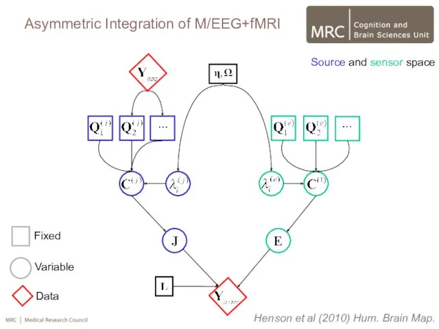
- 52. Henson et al (2010) Hum. Brain Map. Fixed Variable Data Source and sensor space Asymmetric Integration
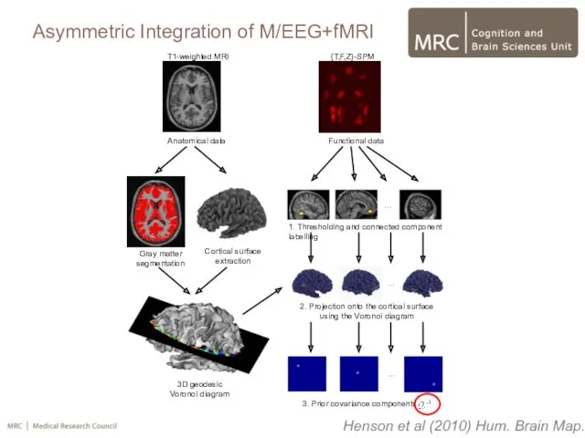
- 53. T1-weighted MRI Anatomical data {T,F,Z}-SPM Gray matter segmentation Cortical surface extraction 3D geodesic Voronoï diagram Functional
- 54. SPM{F} for faces versus scrambled faces, 15 voxels, p 5 clusters from SPM of fMRI data
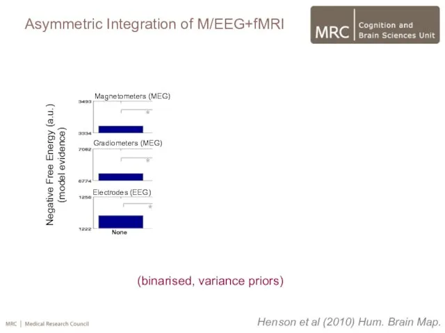
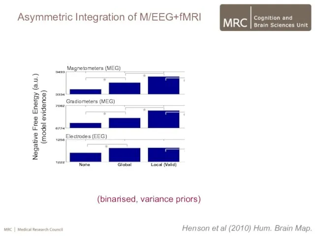
- 55. (binarised, variance priors) Magnetometers (MEG) * * * * None Global Local (Valid) Local (Invalid) Valid+Invalid
- 56. (binarised, variance priors) Magnetometers (MEG) * * * * Gradiometers (MEG) None Global Local (Valid) Local
- 57. (binarised, variance priors) Magnetometers (MEG) * * * * Gradiometers (MEG) None Global Local (Valid) Local
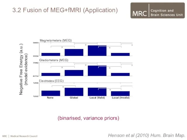
- 58. 3.2 Fusion of MEG+fMRI (Application) (binarised, variance priors) Magnetometers (MEG) * * * * Gradiometers (MEG)
- 59. (binarised, variance priors) Magnetometers (MEG) * * * * Gradiometers (MEG) None Global Local (Valid) Local
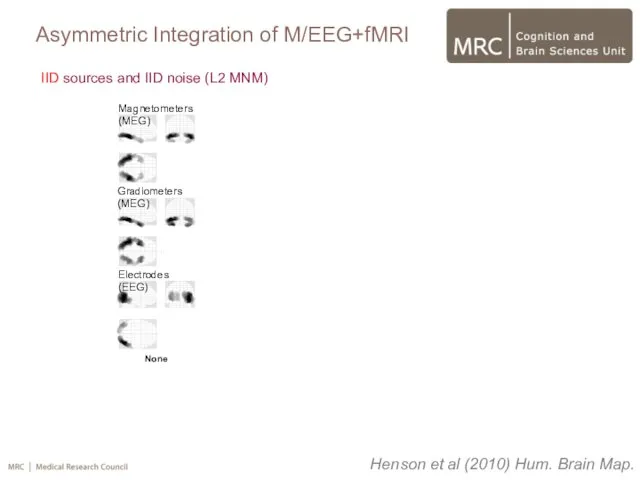
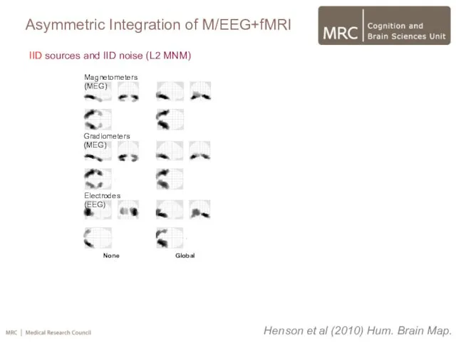
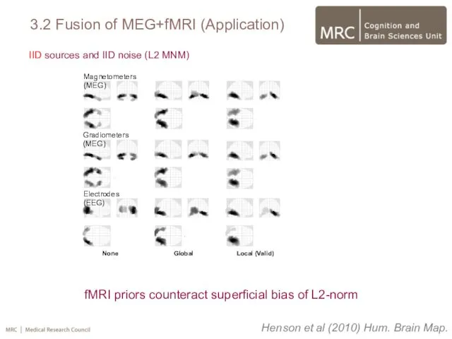
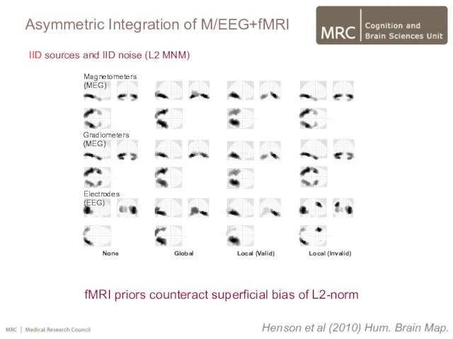
- 60. None Global Local (Valid) Local (Invalid) Magnetometers (MEG) Gradiometers (MEG) Electrodes (EEG) IID sources and IID
- 61. None Global Local (Valid) Local (Invalid) Magnetometers (MEG) Gradiometers (MEG) Electrodes (EEG) IID sources and IID
- 62. 3.2 Fusion of MEG+fMRI (Application) fMRI priors counteract superficial bias of L2-norm None Global Local (Valid)
- 63. fMRI priors counteract superficial bias of L2-norm None Global Local (Valid) Local (Invalid) Magnetometers (MEG) Gradiometers
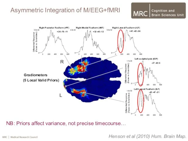
- 64. Prior 4. Prior 5. NB: Priors affect variance, not precise timecourse… R L Gradiometers (MEG) (5
- 65. Adding a single, global fMRI prior increases model evidence Adding multiple valid priors increases model evidence
- 66. Multi-modal Integration 1. Symmetric integration (fusion) of MEG + EEG 2. Asymmetric integration of M/EEG +
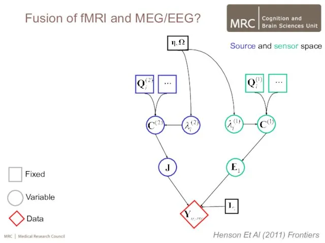
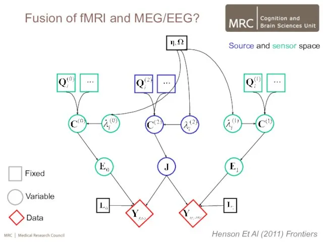
- 67. Fusion of fMRI and MEG/EEG? fMRI MEG ? (future) Data: Causes (hidden): Balloon Model Head Model
- 68. Fusion of fMRI and MEG/EEG? Fixed Variable Data Source and sensor space Henson Et Al (2011)
- 69. Fusion of fMRI and MEG/EEG? Henson Et Al (2011) Frontiers Fixed Variable Data Source and sensor
- 70. Overall Conclusions SPM offers standard forward models (via FieldTrip)… (though with unique option of Canonical Meshes)
- 71. The End
- 72. Likelihood Forward Problem: Physics Ohm’s law: Continuity equation: Maxwell’s Equations: Orientation Location Current (nA):
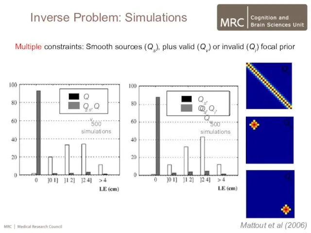
- 73. Inverse Problem: Simulations Mattout et al (2006) Multiple constraints: Smooth sources (Qs), plus valid (Qv) or
- 74. Inverse Problem: Simulations Mattout et al (2006) Multiple constraints: Smooth sources (Qs), plus valid (Qv) or
- 75. Inverse Problem: Temporal Friston et al (2006) V typically Gaussian autocorrelations… In general, temporal correlation of
- 76. Inverse Problem: Temporal Friston et al (2006)
- 77. 3.2. Fusion of MEG+fMRI Prior 4. Prior 5. fMRI hyperparameters ln(λ)+32 ln(λ)+32 Participant Participant Magnetometers (MEG)
- 79. Скачать презентацию
Overview
Forward Models for M/EEG
Variational Bayesian Dipole Estimation (ECD)
Empirical Bayesian Distributed Estimation
Multimodal
Overview
Forward Models for M/EEG
Variational Bayesian Dipole Estimation (ECD)
Empirical Bayesian Distributed Estimation
Multimodal

Overview
Forward Models for M/EEG
Variational Bayesian Dipole Estimation (ECD)
Empirical Bayesian Distributed Estimation
Multimodal
Overview
Forward Models for M/EEG
Variational Bayesian Dipole Estimation (ECD)
Empirical Bayesian Distributed Estimation
Multimodal
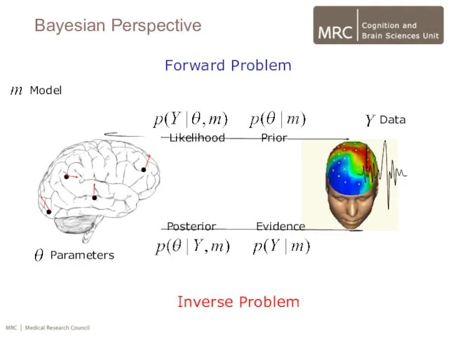
Likelihood Prior
Posterior Evidence
Bayesian Perspective
Forward Problem
Inverse Problem
Data
Parameters
Model
Likelihood Prior
Posterior Evidence
Bayesian Perspective
Forward Problem
Inverse Problem
Data
Parameters
Model
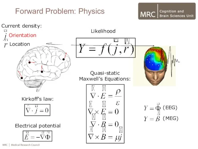
Likelihood
Forward Problem: Physics
Kirkoff’s law:
Electrical potential
Quasi-static
Maxwell’s Equations:
Orientation
Location
Current density:
(EEG)
(MEG)
Likelihood
Forward Problem: Physics
Kirkoff’s law:
Electrical potential
Quasi-static
Maxwell’s Equations:
Orientation
Location
Current density:
(EEG)
(MEG)
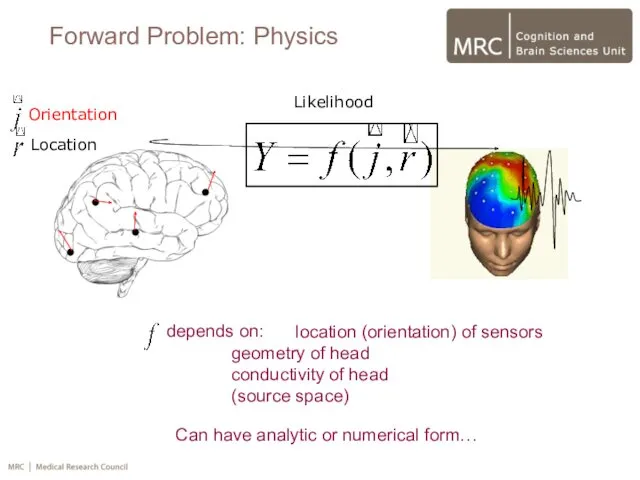
Likelihood
Forward Problem: Physics
Orientation
Location
depends on:
Can have analytic or numerical form…
location (orientation) of
Likelihood
Forward Problem: Physics
Orientation
Location
depends on:
Can have analytic or numerical form…
location (orientation) of

Forward Problem: Head Models
Concentric Spheres:
Pros: Analytic; Fast to compute
Cons: Head
Forward Problem: Head Models
Concentric Spheres:
Pros: Analytic; Fast to compute
Cons: Head
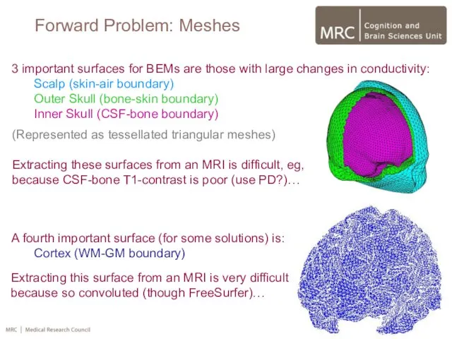
Forward Problem: Meshes
3 important surfaces for BEMs are those with large
Forward Problem: Meshes
3 important surfaces for BEMs are those with large
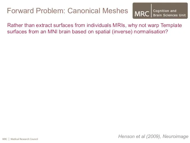
Forward Problem: Canonical Meshes
Rather than extract surfaces from individuals MRIs, why
Forward Problem: Canonical Meshes
Rather than extract surfaces from individuals MRIs, why
fMRI time-series
Motion Correct
Anatomical MRI
Coregister
Deformation
Estimate Spatial Norm
Spatially normalised
Smooth
Smoothed
Template
Recap: (Spatial Normalisation)
fMRI time-series
Motion Correct
Anatomical MRI
Coregister
Deformation
Estimate Spatial Norm
Spatially normalised
Smooth
Smoothed
Template
Recap: (Spatial Normalisation)
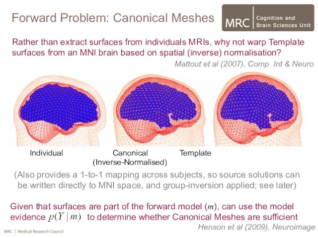
Forward Problem: Canonical Meshes
Rather than extract surfaces from individuals MRIs, why
Forward Problem: Canonical Meshes
Rather than extract surfaces from individuals MRIs, why

Likelihood
Forward Problem: ECD vs Distributed
Orientation
Location
For small number of Equivalent Current Dipoles
Likelihood
Forward Problem: ECD vs Distributed
Orientation
Location
For small number of Equivalent Current Dipoles
Overview
Forward Models for M/EEG
Variational Bayesian Dipole Estimation (ECD)
Empirical Bayesian Distributed Estimation
Multimodal
Overview
Forward Models for M/EEG
Variational Bayesian Dipole Estimation (ECD)
Empirical Bayesian Distributed Estimation
Multimodal
Inverse Problem: VB-ECD
Standard ECD approaches iterate location/orientation (within a brain volume)
Inverse Problem: VB-ECD
Standard ECD approaches iterate location/orientation (within a brain volume)
Inverse Problem: VB-ECD
Maximising the (free-energy approximation to the) model evidence offers
Inverse Problem: VB-ECD
Maximising the (free-energy approximation to the) model evidence offers
Inverse Problem: DCM
Dynamic Causal Modelling (DCM) can be seen as a
Inverse Problem: DCM
Dynamic Causal Modelling (DCM) can be seen as a
Overview
Forward Models for M/EEG
Variational Bayesian Dipole Estimation (ECD)
Empirical Bayesian Distributed Estimation
Multimodal
Overview
Forward Models for M/EEG
Variational Bayesian Dipole Estimation (ECD)
Empirical Bayesian Distributed Estimation
Multimodal
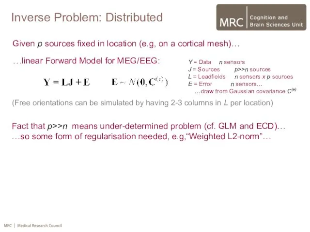
Y = Data n sensors
J = Sources p>>n sources
L = Leadfields n
Y = Data n sensors
J = Sources p>>n sources
L = Leadfields n
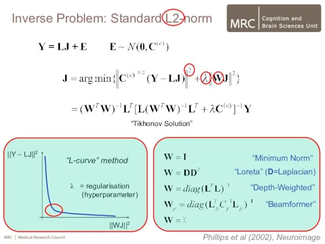
Phillips et al (2002), Neuroimage
Inverse Problem: Standard L2-norm
“Minimum Norm”
“Loreta” (D=Laplacian)
“Depth-Weighted”
“Beamformer”
“Tikhonov Solution”
Phillips et al (2002), Neuroimage
Inverse Problem: Standard L2-norm
“Minimum Norm”
“Loreta” (D=Laplacian)
“Depth-Weighted”
“Beamformer”
“Tikhonov Solution”
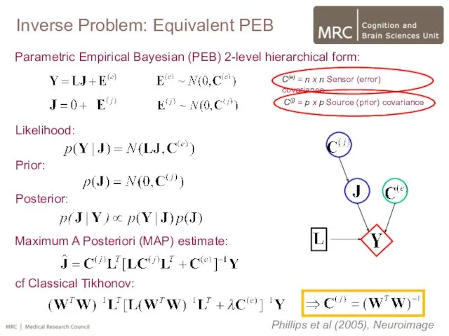
Phillips et al (2005), Neuroimage
Likelihood:
C(e) = n x n Sensor (error)
Phillips et al (2005), Neuroimage
Likelihood:
C(e) = n x n Sensor (error)

Specifying (co)variance components (priors/regularisation):
1. Sensor components, (error):
C = Sensor/Source covariance
Q =
Specifying (co)variance components (priors/regularisation):
1. Sensor components, (error):
C = Sensor/Source covariance
Q =

Henson et al (2007) Neuroimage
When multiple Q’s are correlated, estimation of
Henson et al (2007) Neuroimage
When multiple Q’s are correlated, estimation of
Henson et al (2007) Neuroimage
When multiple Q’s are correlated, estimation of
Henson et al (2007) Neuroimage
When multiple Q’s are correlated, estimation of

Friston et al (2008) Neuroimage
Fixed
Variable
Data
Source and sensor space
Inverse Problem: Full (DAG)
Friston et al (2008) Neuroimage
Fixed
Variable
Data
Source and sensor space
Inverse Problem: Full (DAG)

Friston et al (2002) Neuroimage
1. Obtain Restricted Maximum Likelihood (ReML) estimates
Friston et al (2002) Neuroimage
1. Obtain Restricted Maximum Likelihood (ReML) estimates

Hyperpriors allow the extreme of 100’s source priors, or MSP
Inverse Problem:
Hyperpriors allow the extreme of 100’s source priors, or MSP
Inverse Problem:
Hyperpriors allow the extreme of 100’s source priors, or MSP
Inverse Problem:
Hyperpriors allow the extreme of 100’s source priors, or MSP
Inverse Problem:
Summary:
Automatically “regularises” in principled fashion…
…allows for multiple constraints (priors)…
…to the extent
Summary:
Automatically “regularises” in principled fashion…
…allows for multiple constraints (priors)…
…to the extent
Overview
Forward Models for M/EEG
Variational Bayesian Dipole Estimation (ECD)
Empirical Bayesian Distributed Estimation
Multi-modal
Overview
Forward Models for M/EEG
Variational Bayesian Dipole Estimation (ECD)
Empirical Bayesian Distributed Estimation
Multi-modal
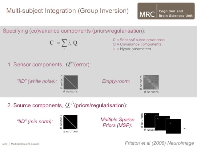
Multi-subject Integration (Group Inversion)
Specifying (co)variance components (priors/regularisation):
1. Sensor components, (error):
C =
Multi-subject Integration (Group Inversion)
Specifying (co)variance components (priors/regularisation):
1. Sensor components, (error):
C =
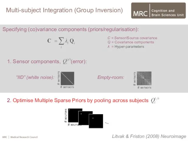
Specifying (co)variance components (priors/regularisation):
1. Sensor components, (error):
C = Sensor/Source covariance
Q =
Specifying (co)variance components (priors/regularisation):
1. Sensor components, (error):
C = Sensor/Source covariance
Q =
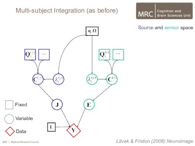
Litvak & Friston (2008) Neuroimage
Fixed
Variable
Data
Source and sensor space
Multi-subject Integration (as before)
Litvak & Friston (2008) Neuroimage
Fixed
Variable
Data
Source and sensor space
Multi-subject Integration (as before)
Litvak & Friston (2008) Neuroimage
Fixed
Variable
Data
Source and sensor space
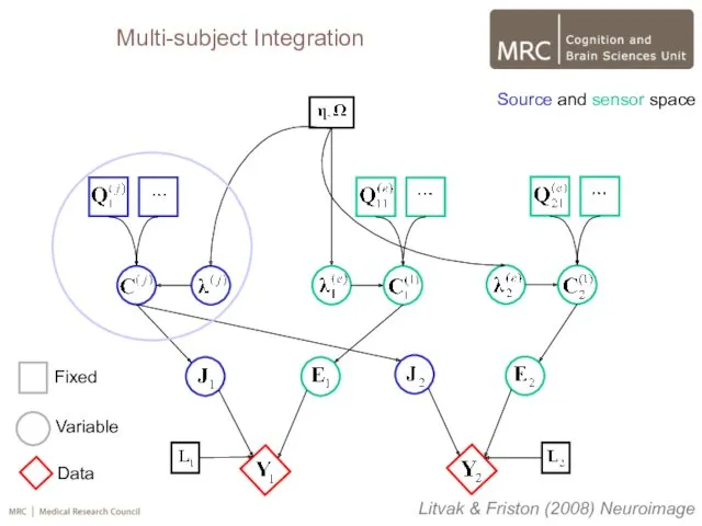
Multi-subject Integration
Litvak & Friston (2008) Neuroimage
Fixed
Variable
Data
Source and sensor space
Multi-subject Integration

Concatenate data across subjects
Common source-level priors:
Subject-specific sensor-level priors:
Litvak & Friston (2008)
Concatenate data across subjects
Common source-level priors:
Subject-specific sensor-level priors:
Litvak & Friston (2008)
Litvak & Friston (2008) Neuroimage
MMN
MSP
MSP (Group)
Multi-subject Integration: Results
Litvak & Friston (2008) Neuroimage
MMN
MSP
MSP (Group)
Multi-subject Integration: Results
Multi-modal Integration
1. Symmetric integration (fusion) of MEG + EEG
2. Asymmetric integration
Multi-modal Integration
1. Symmetric integration (fusion) of MEG + EEG
2. Asymmetric integration
fMRI
MEG
? (future)
Data:
Causes (hidden):
Generative (Forward)
Models:
Balloon
Model
Head
Model
?
EEG
Head
Model
“Neural”
Activity
(inversion)
Multi-modal Integration
Daunizeau et al (2007), Neuroimage
fMRI
MEG
? (future)
Data:
Causes (hidden):
Generative (Forward)
Models:
Balloon
Model
Head
Model
?
EEG
Head
Model
“Neural”
Activity
(inversion)
Multi-modal Integration
Daunizeau et al (2007), Neuroimage

Asymmetric
Integration
fMRI
MEG
? (future)
Data:
Causes (hidden):
Generative (Forward)
Models:
Balloon
Model
Head
Model
?
EEG
Head
Model
“Neural”
Activity
Symmetric
Integration
(Fusion)
Daunizeau et al (2007), Neuroimage
Multi-modal Integration
Asymmetric
Integration
fMRI
MEG
? (future)
Data:
Causes (hidden):
Generative (Forward)
Models:
Balloon
Model
Head
Model
?
EEG
Head
Model
“Neural”
Activity
Symmetric
Integration
(Fusion)
Daunizeau et al (2007), Neuroimage
Multi-modal Integration

Multi-modal Integration
1. Symmetric integration (fusion) of MEG + EEG
2. Asymmetric integration
Multi-modal Integration
1. Symmetric integration (fusion) of MEG + EEG
2. Asymmetric integration
Specifying (co)variance components (priors/regularisation):
1. Sensor components, (error):
C = Sensor/Source covariance
Q =
Specifying (co)variance components (priors/regularisation):
1. Sensor components, (error):
C = Sensor/Source covariance
Q =

Specifying (co)variance components (priors/regularisation):
1. Sensor components, (error):
Ci(e) = Sensor error covariance for
Specifying (co)variance components (priors/regularisation):
1. Sensor components, (error):
Ci(e) = Sensor error covariance for
Henson et al (2009) Neuroimage
Fixed
Variable
Data
Source and sensor space
Single Modality (as before)
Henson et al (2009) Neuroimage
Fixed
Variable
Data
Source and sensor space
Single Modality (as before)
Henson et al (2009) Neuroimage
Fixed
Variable
Data
Source and sensor space
Multiple modalities
Henson et al (2009) Neuroimage
Fixed
Variable
Data
Source and sensor space
Multiple modalities
Henson et al (2009) Neuroimage
Stack data and leadfields for d modalities:
Where
Henson et al (2009) Neuroimage
Stack data and leadfields for d modalities:
Where
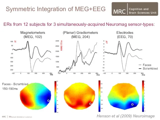
ERs from 12 subjects for 3 simultaneously-acquired Neuromag sensor-types:
RMS fT/m
μV
Faces
Scrambled
fT
Magnetometers
(MEG,
ERs from 12 subjects for 3 simultaneously-acquired Neuromag sensor-types:
RMS fT/m
μV
Faces
Scrambled
fT
Magnetometers
(MEG,
MEG mags
MEG grads
EEG
FUSED
+31
MEG mags
MEG grads
EEG
FUSED
+31
Henson et al (2009) Neuroimage
Fusing magnetometers, gradiometers and EEG increased the
Henson et al (2009) Neuroimage
Fusing magnetometers, gradiometers and EEG increased the
Multi-modal Integration
1. Symmetric integration (fusion) of MEG + EEG
2. Asymmetric integration
Multi-modal Integration
1. Symmetric integration (fusion) of MEG + EEG
2. Asymmetric integration

Asymmetric Integration of M/EEG+fMRI
Specifying (co)variance components (priors/regularisation):
1. Sensor components, (error):
C
Asymmetric Integration of M/EEG+fMRI
Specifying (co)variance components (priors/regularisation):
1. Sensor components, (error):
C
Henson et al (2010) Hum. Brain Map.
Specifying (co)variance components (priors/regularisation):
1. Sensor
Henson et al (2010) Hum. Brain Map.
Specifying (co)variance components (priors/regularisation):
1. Sensor

Friston et al (2008) Neuroimage
Fixed
Variable
Data
Source and sensor space
Asymmetric Integration of M/EEG+fMRI
Friston et al (2008) Neuroimage
Fixed
Variable
Data
Source and sensor space
Asymmetric Integration of M/EEG+fMRI
Henson et al (2010) Hum. Brain Map.
Fixed
Variable
Data
Source and sensor space
Asymmetric Integration
Henson et al (2010) Hum. Brain Map.
Fixed
Variable
Data
Source and sensor space
Asymmetric Integration
T1-weighted MRI
Anatomical data
{T,F,Z}-SPM
Gray matter
segmentation
Cortical surface
extraction
3D geodesic
Voronoï diagram
Functional data
…
1. Thresholding and
T1-weighted MRI
Anatomical data
{T,F,Z}-SPM
Gray matter
segmentation
Cortical surface
extraction
3D geodesic
Voronoï diagram
Functional data
…
1. Thresholding and
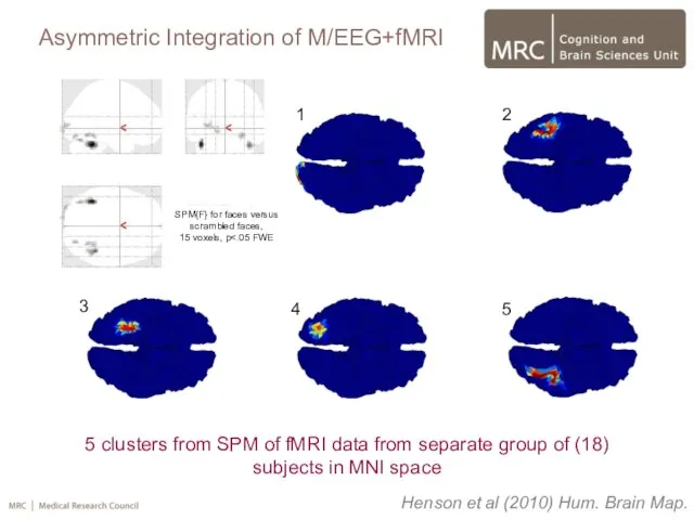
SPM{F} for faces versus scrambled faces,
15 voxels, p<.05 FWE
5 clusters
SPM{F} for faces versus scrambled faces,
15 voxels, p<.05 FWE
5 clusters
(binarised, variance priors)
Magnetometers (MEG)
*
*
*
*
None Global Local (Valid) Local (Invalid)
(binarised, variance priors)
Magnetometers (MEG)
*
*
*
*
None Global Local (Valid) Local (Invalid)

(binarised, variance priors)
Magnetometers (MEG)
*
*
*
*
Gradiometers (MEG)
None Global Local (Valid)
(binarised, variance priors)
Magnetometers (MEG)
*
*
*
*
Gradiometers (MEG)
None Global Local (Valid)
(binarised, variance priors)
Magnetometers (MEG)
*
*
*
*
Gradiometers (MEG)
None Global Local (Valid)
(binarised, variance priors)
Magnetometers (MEG)
*
*
*
*
Gradiometers (MEG)
None Global Local (Valid)
3.2 Fusion of MEG+fMRI (Application)
(binarised, variance priors)
Magnetometers (MEG)
*
*
*
*
Gradiometers (MEG)
3.2 Fusion of MEG+fMRI (Application)
(binarised, variance priors)
Magnetometers (MEG)
*
*
*
*
Gradiometers (MEG)

(binarised, variance priors)
Magnetometers (MEG)
*
*
*
*
Gradiometers (MEG)
None Global Local (Valid)
(binarised, variance priors)
Magnetometers (MEG)
*
*
*
*
Gradiometers (MEG)
None Global Local (Valid)
None Global Local (Valid) Local (Invalid)
Magnetometers (MEG)
Gradiometers (MEG)
Electrodes (EEG)
IID
None Global Local (Valid) Local (Invalid)
Magnetometers (MEG)
Gradiometers (MEG)
Electrodes (EEG)
IID
None Global Local (Valid) Local (Invalid)
Magnetometers (MEG)
Gradiometers (MEG)
Electrodes (EEG)
IID
None Global Local (Valid) Local (Invalid)
Magnetometers (MEG)
Gradiometers (MEG)
Electrodes (EEG)
IID
3.2 Fusion of MEG+fMRI (Application)
fMRI priors counteract superficial bias of L2-norm
3.2 Fusion of MEG+fMRI (Application)
fMRI priors counteract superficial bias of L2-norm
fMRI priors counteract superficial bias of L2-norm
None Global Local (Valid)
fMRI priors counteract superficial bias of L2-norm
None Global Local (Valid)
Prior 4.
Prior 5.
NB: Priors affect variance, not precise timecourse…
R
L
Gradiometers (MEG)
(5 Local
Prior 4.
Prior 5.
NB: Priors affect variance, not precise timecourse…
R
L
Gradiometers (MEG)
(5 Local
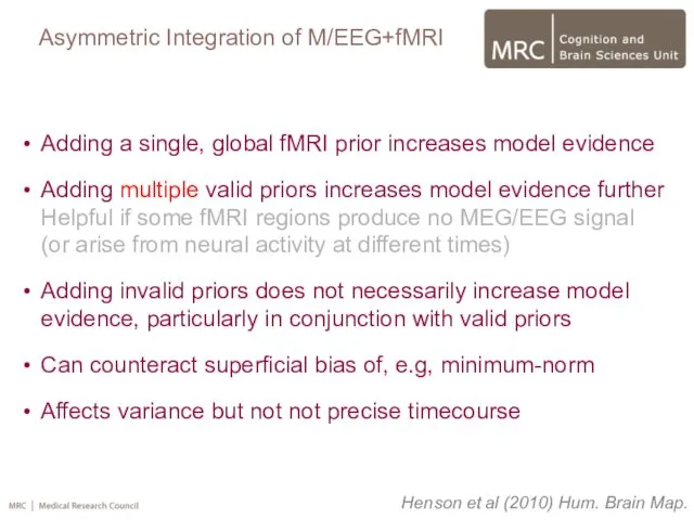
Adding a single, global fMRI prior increases model evidence
Adding multiple valid
Adding a single, global fMRI prior increases model evidence
Adding multiple valid

Multi-modal Integration
1. Symmetric integration (fusion) of MEG + EEG
2. Asymmetric integration
Multi-modal Integration
1. Symmetric integration (fusion) of MEG + EEG
2. Asymmetric integration

Fusion of fMRI and MEG/EEG?
fMRI
MEG
? (future)
Data:
Causes (hidden):
Balloon
Model
Head
Model
?
EEG
Head
Model
“Neural”
Activity
Fusion of
Fusion of fMRI and MEG/EEG?
fMRI
MEG
? (future)
Data:
Causes (hidden):
Balloon
Model
Head
Model
?
EEG
Head
Model
“Neural”
Activity
Fusion of
Fusion of fMRI and MEG/EEG?
Fixed
Variable
Data
Source and sensor space
Henson Et Al
Fusion of fMRI and MEG/EEG?
Fixed
Variable
Data
Source and sensor space
Henson Et Al
Fusion of fMRI and MEG/EEG?
Henson Et Al (2011) Frontiers
Fixed
Variable
Data
Source and
Fusion of fMRI and MEG/EEG?
Henson Et Al (2011) Frontiers
Fixed
Variable
Data
Source and
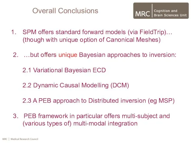
Overall Conclusions
SPM offers standard forward models (via FieldTrip)…
(though with unique option
Overall Conclusions
SPM offers standard forward models (via FieldTrip)…
(though with unique option

The End
The End
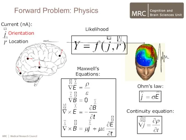
Likelihood
Forward Problem: Physics
Ohm’s law:
Continuity equation:
Maxwell’s
Equations:
Orientation
Location
Current (nA):
Likelihood
Forward Problem: Physics
Ohm’s law:
Continuity equation:
Maxwell’s
Equations:
Orientation
Location
Current (nA):
Inverse Problem: Simulations
Mattout et al (2006)
Multiple constraints: Smooth sources (Qs), plus
Inverse Problem: Simulations
Mattout et al (2006)
Multiple constraints: Smooth sources (Qs), plus

Inverse Problem: Simulations
Mattout et al (2006)
Multiple constraints: Smooth sources (Qs), plus
Inverse Problem: Simulations
Mattout et al (2006)
Multiple constraints: Smooth sources (Qs), plus

Inverse Problem: Temporal
Friston et al (2006)
V typically Gaussian autocorrelations…
In general,
Inverse Problem: Temporal
Friston et al (2006)
V typically Gaussian autocorrelations…
In general,

Inverse Problem: Temporal
Friston et al (2006)
Inverse Problem: Temporal
Friston et al (2006)

3.2. Fusion of MEG+fMRI
Prior 4.
Prior 5.
fMRI hyperparameters
ln(λ)+32
ln(λ)+32
Participant
Participant
Magnetometers (MEG)
Gradiometers (MEG)
Electrodes (EEG)
Local
Valid
Local
3.2. Fusion of MEG+fMRI
Prior 4.
Prior 5.
fMRI hyperparameters
ln(λ)+32
ln(λ)+32
Participant
Participant
Magnetometers (MEG)
Gradiometers (MEG)
Electrodes (EEG)
Local
Valid
Local
 Применение динамических массивов в структурном подходе
 Короткий текст. Структура новости
 Internet-игрушка, помощник или враг?
 Функциональное и доменное тестирование
 Построение диаграмм и графиков
 Интеллектуально-развлекательная игра Science quiz
 Microstrategy visualization guidelines
 Урок-обобщение по теме Устройства ПК
 Текстовий процесор. (8 класс)
 Урок В мире кодов
 Компоненты в React. Урок №1
 Microsoft Office. Программы
 Автоматизоване створення веб-сайту
 Операциялық жүйе үзілістерін өңдеу
 Новые профессии и специальности, связанные с Интернетом
 Paint графикалық редакторы
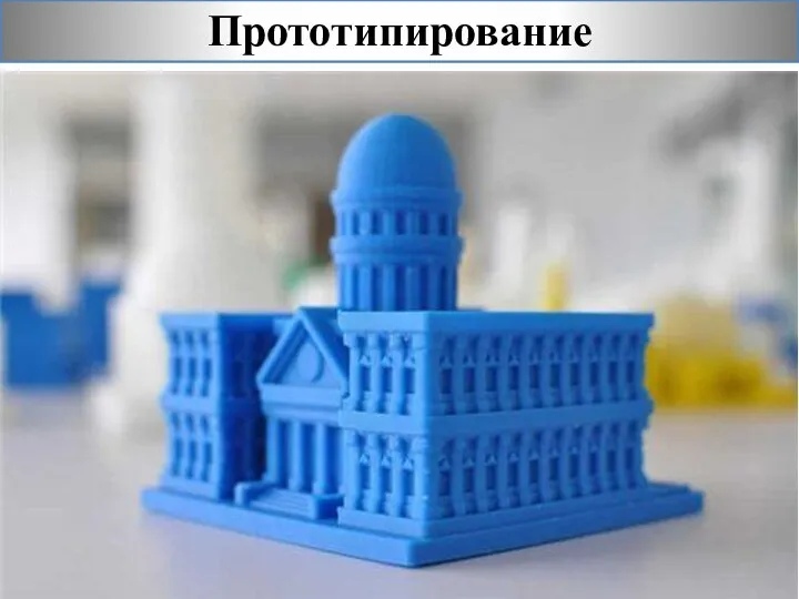 Прототипирование и 3D печать
 Современные технологии разработки программного обеспечения
 : Обработка ирнформации
 Техника безопасности при обслуживании информационных систем
 Таймлайн искусственных нейронных сетей
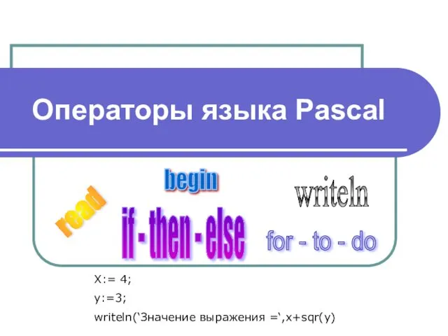 Операторы языка Pascal
 Информационная безопасность предприятия
 Ввод и вывод
 Табличные процессоры (тема 4)
 Программное обеспечение персонального компьютера. Операционная система
 Опыт работы по теме Информационно-коммуникационные технологии, как одно из средств познавательного развития детей дошкольного возраста
 Алгоритмы оптимизации