- The travelling salesman problem

Содержание
- 2. The origins of the travelling salesman problem are unclear The travelling salesman problem was mathematically formulated
- 3. It was first considered mathematically in the 1930s by Merrill Flood who was looking to solve
- 4. History In the 1950s and 1960s, the problem became increasingly popular in scientific circles in Europe
- 5. As a graph problem TSP can be modelled as an undirected weighted graph, such that cities
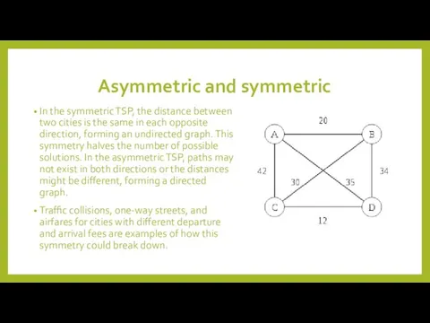
- 6. Asymmetric and symmetric In the symmetric TSP, the distance between two cities is the same in
- 7. Related problems An equivalent formulation in terms of graph theory is: Given a complete weighted graph
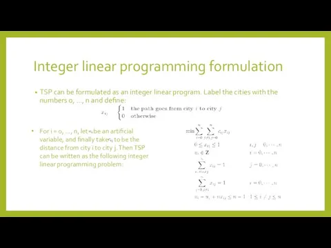
- 8. Integer linear programming formulation TSP can be formulated as an integer linear program. Label the cities
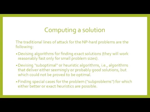
- 9. Computing a solution The traditional lines of attack for the NP-hard problems are the following: Devising
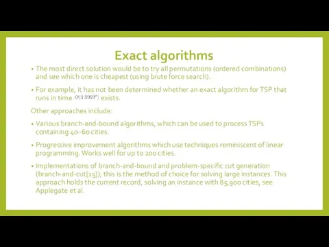
- 10. Exact algorithms The most direct solution would be to try all permutations (ordered combinations) and see
- 11. Exact algorithms
- 12. Heuristic and approximation algorithms Various heuristics and approximation algorithms, which quickly yield good solutions have been
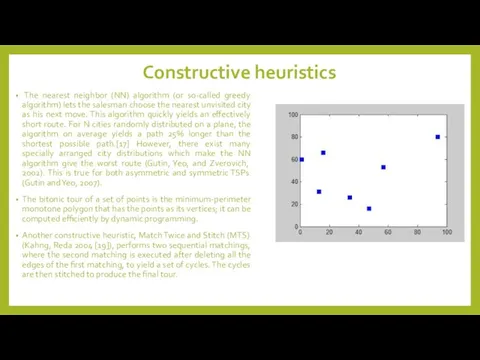
- 13. Constructive heuristics The nearest neighbor (NN) algorithm (or so-called greedy algorithm) lets the salesman choose the
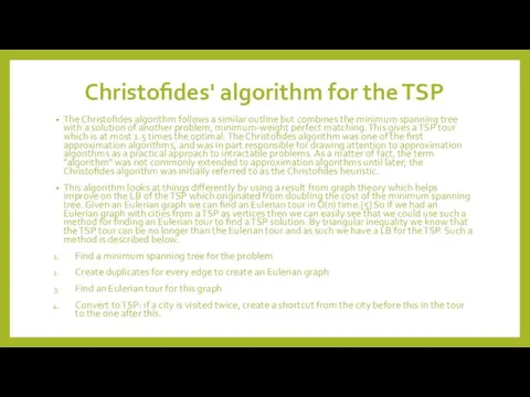
- 14. Christofides' algorithm for the TSP The Christofides algorithm follows a similar outline but combines the minimum
- 15. Using a shortcut heuristic on the graph created by the matching below
- 16. Iterative improvement Pairwise exchange The pairwise exchange or 2-opt technique involves iteratively removing two edges and
- 17. Randomised improvement Optimized Markov chain algorithms which use local searching heuristic sub-algorithms can find a route
- 18. Ant colony optimization Artificial intelligence researcher Marco Dorigo described in 1993 a method of heuristically generating
- 19. Special cases of the TSP Metric TSP In the metric TSP, also known as delta-TSP or
- 20. Asymmetric TSP In most cases, the distance between two nodes in the TSP network is the
- 21. Analyst's travelling salesman problem There is an analogous problem in geometric measure theory which asks the
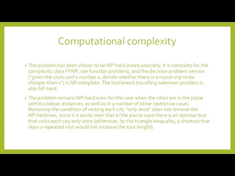
- 22. Computational complexity The problem has been shown to be NP-hard (more precisely, it is complete for
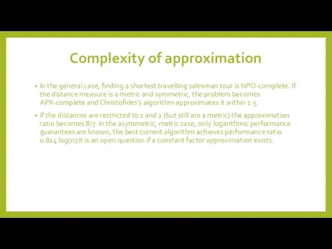
- 23. Complexity of approximation In the general case, finding a shortest travelling salesman tour is NPO-complete. If
- 25. Скачать презентацию
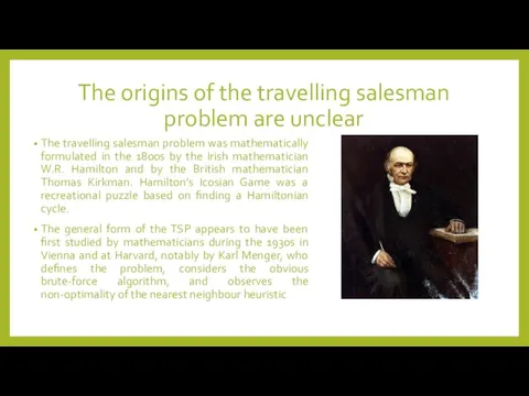
The origins of the travelling salesman problem are unclear
The travelling salesman
The origins of the travelling salesman problem are unclear
The travelling salesman
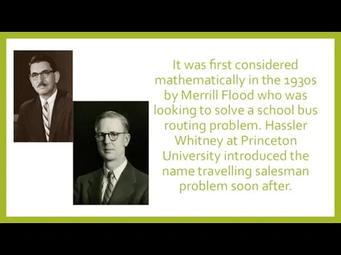
It was first considered mathematically in the 1930s by Merrill Flood
It was first considered mathematically in the 1930s by Merrill Flood
History
In the 1950s and 1960s, the problem became increasingly popular in
History
In the 1950s and 1960s, the problem became increasingly popular in
As a graph problem
TSP can be modelled as an undirected weighted
As a graph problem
TSP can be modelled as an undirected weighted
Asymmetric and symmetric
In the symmetric TSP, the distance between two cities
Asymmetric and symmetric
In the symmetric TSP, the distance between two cities
Related problems
An equivalent formulation in terms of graph theory is: Given
Related problems
An equivalent formulation in terms of graph theory is: Given
Integer linear programming formulation
TSP can be formulated as an integer linear
Integer linear programming formulation
TSP can be formulated as an integer linear
Computing a solution
The traditional lines of attack for the NP-hard problems
Computing a solution
The traditional lines of attack for the NP-hard problems
Exact algorithms
The most direct solution would be to try all permutations
Exact algorithms
The most direct solution would be to try all permutations
Exact algorithms
Exact algorithms
Heuristic and approximation algorithms
Various heuristics and approximation algorithms, which quickly yield
Heuristic and approximation algorithms
Various heuristics and approximation algorithms, which quickly yield
Constructive heuristics
The nearest neighbor (NN) algorithm (or so-called greedy algorithm)
Constructive heuristics
The nearest neighbor (NN) algorithm (or so-called greedy algorithm)
Christofides' algorithm for the TSP
The Christofides algorithm follows a similar outline
Christofides' algorithm for the TSP
The Christofides algorithm follows a similar outline
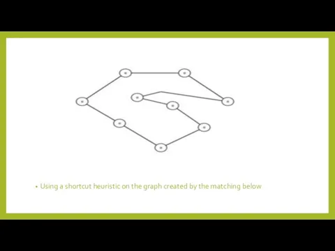
Using a shortcut heuristic on the graph created by the matching
Using a shortcut heuristic on the graph created by the matching
Iterative improvement
Pairwise exchange
The pairwise exchange or 2-opt technique involves iteratively removing
Iterative improvement
Pairwise exchange
The pairwise exchange or 2-opt technique involves iteratively removing
Randomised improvement
Optimized Markov chain algorithms which use local searching heuristic sub-algorithms
Randomised improvement
Optimized Markov chain algorithms which use local searching heuristic sub-algorithms
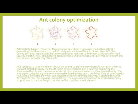
Ant colony optimization
Artificial intelligence researcher Marco Dorigo described in 1993 a
Ant colony optimization
Artificial intelligence researcher Marco Dorigo described in 1993 a
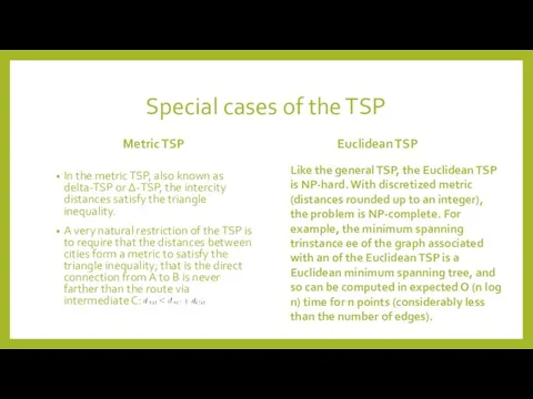
Special cases of the TSP
Metric TSP
In the metric TSP, also known
Special cases of the TSP
Metric TSP
In the metric TSP, also known
Asymmetric TSP
In most cases, the distance between two nodes in the
Asymmetric TSP
In most cases, the distance between two nodes in the
Analyst's travelling salesman problem
There is an analogous problem in geometric measure
Analyst's travelling salesman problem
There is an analogous problem in geometric measure
Computational complexity
The problem has been shown to be NP-hard (more precisely,
Computational complexity
The problem has been shown to be NP-hard (more precisely,
Complexity of approximation
In the general case, finding a shortest travelling salesman
Complexity of approximation
In the general case, finding a shortest travelling salesman
 Radix sort
 Объемы тел
 Разминка. Быстрее. Выше. Сильнее
 Математика в 3 классе
 Теория вероятностей
 Геометрия куполов
 Тренажёр к уроку геометрии в 7 классе. УМК Геометрия 7-9. Атанасян Л.С
 Векторы и прямые произведения множеств. Проекция вектора на ось
 Математические тесты
 Устный журнал по математике
 Аполлоній Перзький
 Перпендикулярность прямых и плоскостей
 Изменение величин
 Первообразная. Неопределенный интеграл
 Решение геометрических задач при подготовке к ГИА
 Trigonometry 4. Lecture Outline
 Презентация Площадь геометрической фигуры
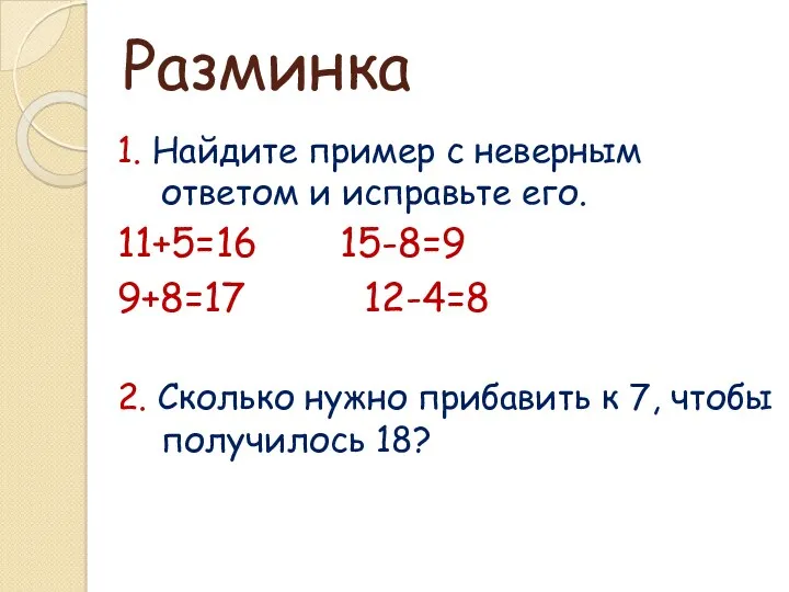 Устный счёт 1 класс
 Внеклассное мероприятие по математике Своя игра (для учащихся 5-х классов)
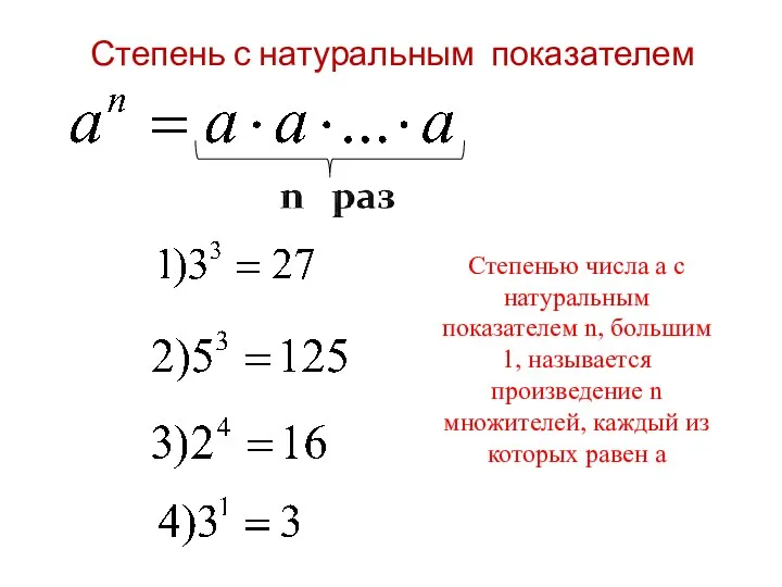 Степень с натуральным показателем. Умножение степеней с одинаковыми а основаниями
 Задачи на движение
 Обобщающий урок по теме Четырёхугольники.
 Понятие квадратного корня из неотрицательного числа
 Что есть угол? Математика. Лекция №6
 Урок математики
 Теория комплексных чисел. (Тема 2)
 Элементы теории матричных игр
 Методическое пособие по развитию сенсорных представлений, развитие внимания, памяти, мышления