- Winston p. 313

Содержание
- 2. Winston p. 313, # 2 Dual: min 3y1 + 2y2 + y3 subject to y1 +
- 3. Winston p. 815, #11 Find the floor and ceiling of the value of this game. Does
- 4. Winston p. 815, #11 min -1 -10 -10 -1 -10 max 20 20 -1 7 2
- 5. Schrage #4 The next 5 slides show the crop recourse homework problem I assigned, plus the
- 6. Schrage #4 (Formulate Only)
- 7. Schrage Handout, #4 Indices s = season {wet,dry} c = crops {corn, sorg, bean} Data YIELDcs
- 8. Schrage Handout, #4 (cont’d)
- 9. Schrage #4 (Sample MPL Code) TITLE RecourseCrops; INDEX s := (wet,dry); { seasons } c :=
- 10. Schrage #4 (Sample MPL code) DECISION VARIABLES live; { units of livestock to raise } pcrop[c];
- 12. Скачать презентацию
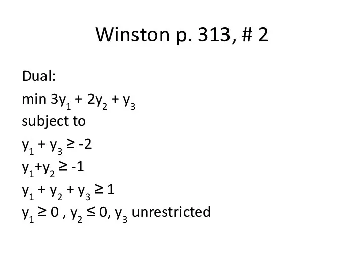
Winston p. 313, # 2
Dual:
min 3y1 + 2y2 + y3
subject to
y1
Winston p. 313, # 2
Dual:
min 3y1 + 2y2 + y3
subject to
y1
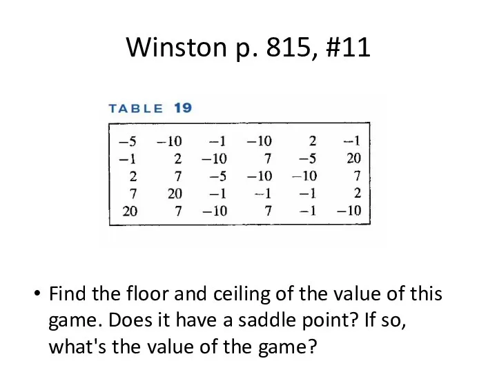
Winston p. 815, #11
Find the floor and ceiling of the value
Winston p. 815, #11
Find the floor and ceiling of the value
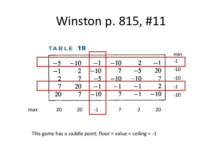
Winston p. 815, #11
min
-1
-10
-10
-1
-10
max 20 20 -1 7 2 20
This game
Winston p. 815, #11
min
-1
-10
-10
-1
-10
max 20 20 -1 7 2 20
This game
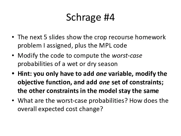
Schrage #4
The next 5 slides show the crop recourse homework problem
Schrage #4
The next 5 slides show the crop recourse homework problem
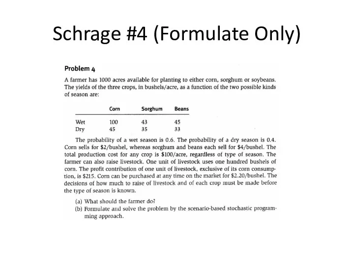
Schrage #4 (Formulate Only)
Schrage #4 (Formulate Only)
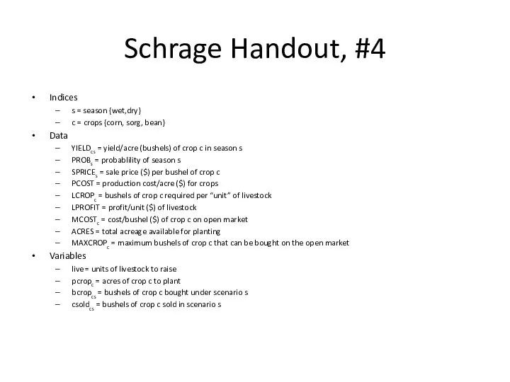
Schrage Handout, #4
Indices
s = season {wet,dry}
c = crops {corn, sorg, bean}
Data
YIELDcs
Schrage Handout, #4
Indices
s = season {wet,dry}
c = crops {corn, sorg, bean}
Data
YIELDcs
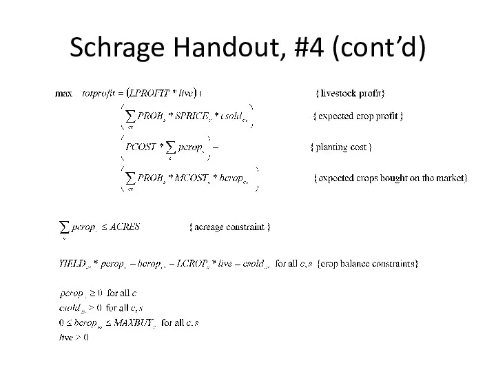
Schrage Handout, #4 (cont’d)
Schrage Handout, #4 (cont’d)
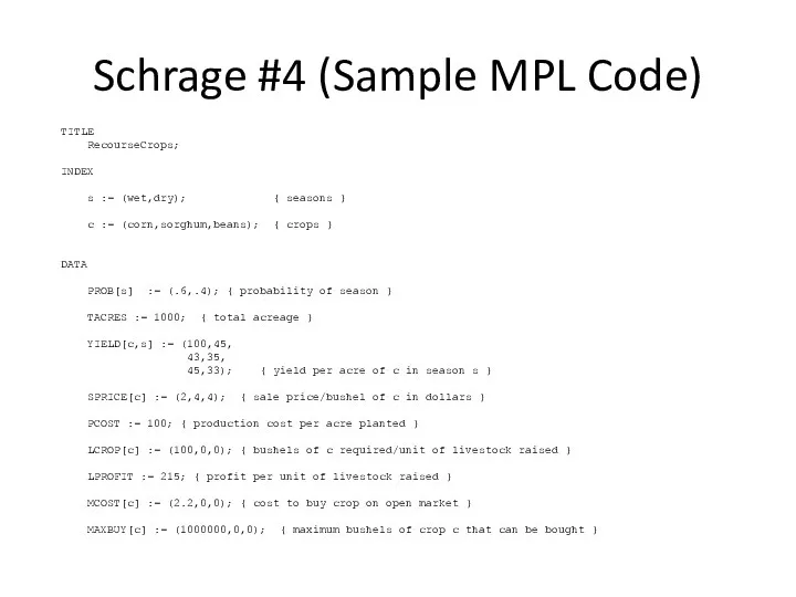
Schrage #4 (Sample MPL Code)
TITLE
RecourseCrops;
INDEX
s := (wet,dry); { seasons
Schrage #4 (Sample MPL Code)
TITLE
RecourseCrops;
INDEX
s := (wet,dry); { seasons
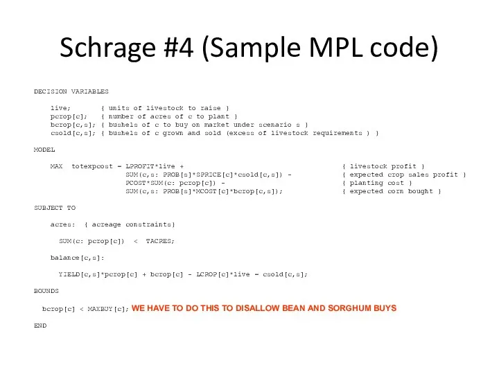
Schrage #4 (Sample MPL code)
DECISION VARIABLES
live; { units of livestock
Schrage #4 (Sample MPL code)
DECISION VARIABLES
live; { units of livestock
 Предел числовой последовательности. Способы задания числовой последовательности
 Линейная функция и её график
 Задачи теории вероятностей. Повторение к ГИА и ЕГЭ
 Вынесение общего множителя
 Урок Весёлый математик - 2 класс
 Сравнение, сложение и вычитание дробей с разными знаменателями
 Умножение и деление на 9
 Свойства логарифмов. Джон Непер (1550-1617)
 Решение задач на движение
 Векторное произведение векторов
 презентация КВМ внеклассное мероприятие по математике 4 класс
 Презентация к уроку закрепление умножение и деление на 2
 10 способов решения квадратных уравнений
 Мәтінді есептерді шығару
 презентация Числа от 1 до 7
 Определение степени с целым отрицательным показателем. 8 класс
 Алгебра. Исторический очерк
 Деление суммы на число
 Выражение. Составь выражение
 Сложение и вычитание алгебраических дробей с разными знаменателями
 презентация по математике Табличное умножение и деление 2 класс
 Линейная алгебра. Матрицы
 Двусвязность. (Лекция 7)
 Физминутка в картинках
 Определённый интеграл
 Слагаемое. Компоненты при умножении
 Сложение однозначных чисел с переходом через десяток
 Пропорции» и «Прямая и обратная пропорциональность