- Price Equilibrium 11.2a

Содержание
- 2. Learning Objectives By the end of the lesson the learners will be able to : Define
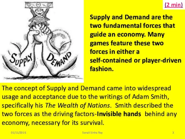
- 3. 01/11/2016 Sonali Sinha Roy Supply and Demand are the two fundamental forces that guide an economy.
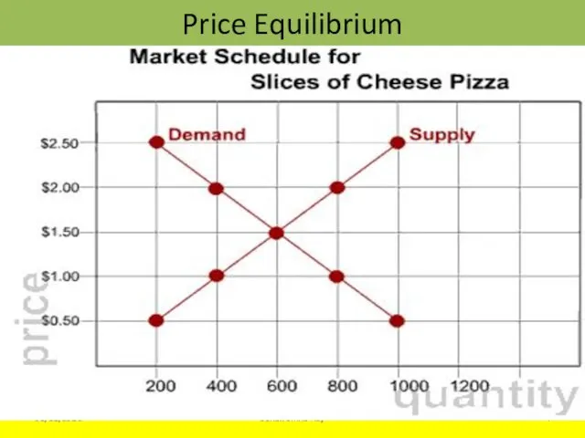
- 4. 01/11/2016 Sonali Sinha Roy Price Equilibrium
- 5. Price Equilibrium 01/11/2016 Sonali Sinha Roy
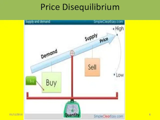
- 6. 01/11/2016 Sonali Sinha Roy Price Disequilibrium
- 7. Excess Demand/ Shortage 01/11/2016 Sonali Sinha Roy
- 8. Excess Supply/Surplus 01/11/2016 Sonali Sinha Roy
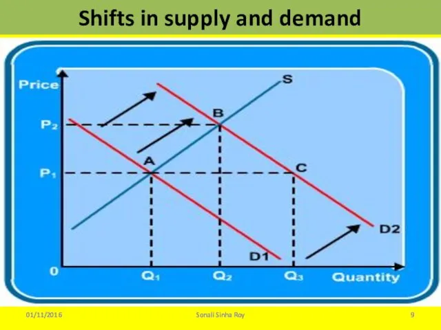
- 9. Shifts in supply and demand 01/11/2016 Sonali Sinha Roy
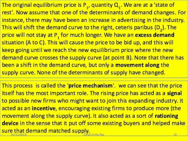
- 10. 01/11/2016 Sonali Sinha Roy The original equilibrium price is P1, quantity Q1. We are at a
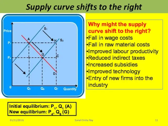
- 11. Supply curve shifts to the right 01/11/2016 Sonali Sinha Roy Why might the supply curve shift
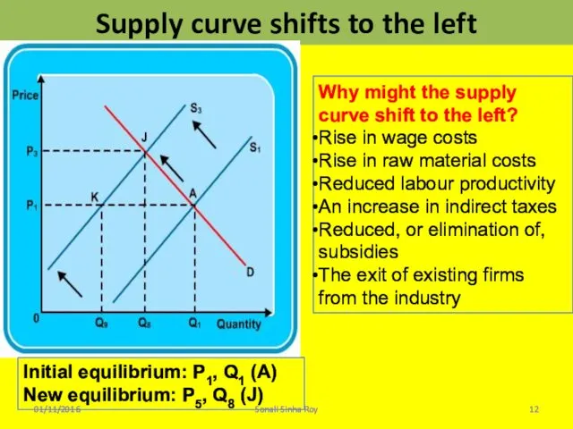
- 12. Supply curve shifts to the left 01/11/2016 Sonali Sinha Roy Why might the supply curve shift
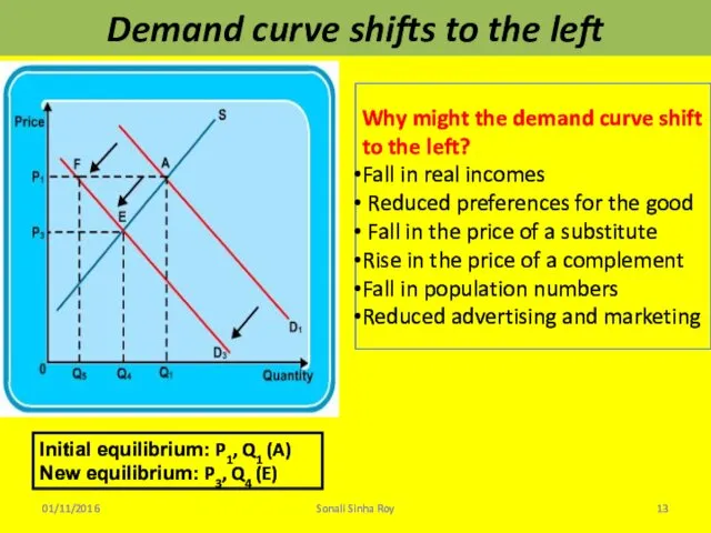
- 13. Demand curve shifts to the left 01/11/2016 Sonali Sinha Roy Why might the demand curve shift
- 14. 01/11/2016 Sonali Sinha Roy New Price Equilibrium
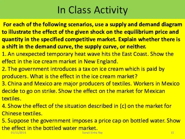
- 15. In Class Activity 01/11/2016 Sonali Sinha Roy For each of the following scenarios, use a supply
- 16. Recap of Today’s Lesson 01/11/2016 Sonali Sinha Roy
- 17. Reflection 01/11/2016 Sonali Sinha Roy
- 18. Price Equilibrium function 11.2a Lesson 6 NIS 01/11/2016 Sonali Sinha Roy
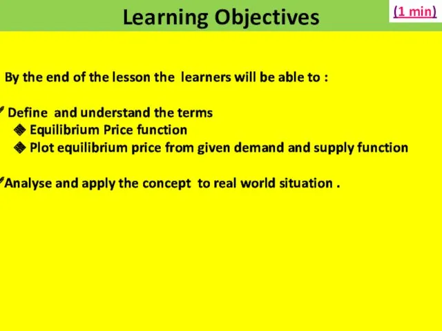
- 19. Learning Objectives By the end of the lesson the learners will be able to : Define
- 20. Equilibrium Price Function Demand Function Qd = a – bP Qd = quantity of a good
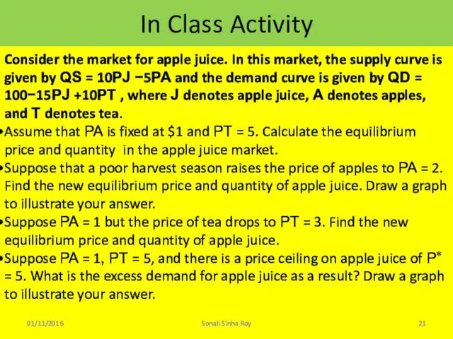
- 21. In Class Activity 01/11/2016 Sonali Sinha Roy Consider the market for apple juice. In this market,
- 22. Recap of Today’s Lesson 01/11/2016 Sonali Sinha Roy
- 24. Скачать презентацию
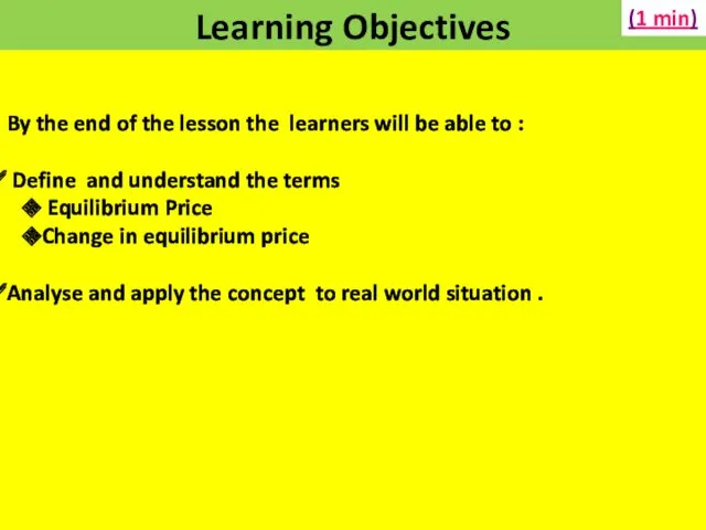
Learning Objectives
By the end of the lesson the learners will
Learning Objectives
By the end of the lesson the learners will
01/11/2016
Sonali Sinha Roy
Supply and Demand are the two fundamental forces that
01/11/2016
Sonali Sinha Roy
Supply and Demand are the two fundamental forces that
01/11/2016
Sonali Sinha Roy
Price Equilibrium
01/11/2016
Sonali Sinha Roy
Price Equilibrium
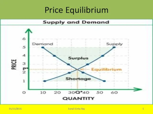
Price Equilibrium
01/11/2016
Sonali Sinha Roy
Price Equilibrium
01/11/2016
Sonali Sinha Roy
01/11/2016
Sonali Sinha Roy
Price Disequilibrium
01/11/2016
Sonali Sinha Roy
Price Disequilibrium
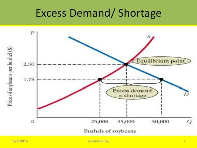
Excess Demand/ Shortage
01/11/2016
Sonali Sinha Roy
Excess Demand/ Shortage
01/11/2016
Sonali Sinha Roy
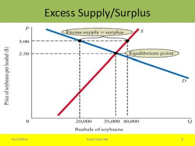
Excess Supply/Surplus
01/11/2016
Sonali Sinha Roy
Excess Supply/Surplus
01/11/2016
Sonali Sinha Roy
Shifts in supply and demand
01/11/2016
Sonali Sinha Roy
Shifts in supply and demand
01/11/2016
Sonali Sinha Roy
01/11/2016
Sonali Sinha Roy
The original equilibrium price is P1, quantity Q1. We
01/11/2016
Sonali Sinha Roy
The original equilibrium price is P1, quantity Q1. We
Supply curve shifts to the right
01/11/2016
Sonali Sinha Roy
Why might the supply
Supply curve shifts to the right
01/11/2016
Sonali Sinha Roy
Why might the supply
Supply curve shifts to the left
01/11/2016
Sonali Sinha Roy
Why might the supply
Supply curve shifts to the left
01/11/2016
Sonali Sinha Roy
Why might the supply
Demand curve shifts to the left
01/11/2016
Sonali Sinha Roy
Why might the demand
Demand curve shifts to the left
01/11/2016
Sonali Sinha Roy
Why might the demand

01/11/2016
Sonali Sinha Roy
New Price Equilibrium
01/11/2016
Sonali Sinha Roy
New Price Equilibrium
In Class Activity
01/11/2016
Sonali Sinha Roy
For each of the following scenarios,
In Class Activity
01/11/2016
Sonali Sinha Roy
For each of the following scenarios,
Recap of Today’s Lesson
01/11/2016
Sonali Sinha Roy
Recap of Today’s Lesson
01/11/2016
Sonali Sinha Roy

Reflection
01/11/2016
Sonali Sinha Roy
Reflection
01/11/2016
Sonali Sinha Roy
Price Equilibrium function
11.2a
Lesson 6
NIS
01/11/2016
Sonali Sinha Roy
Price Equilibrium function
11.2a
Lesson 6
NIS
01/11/2016
Sonali Sinha Roy
Learning Objectives
By the end of the lesson the learners will
Learning Objectives
By the end of the lesson the learners will
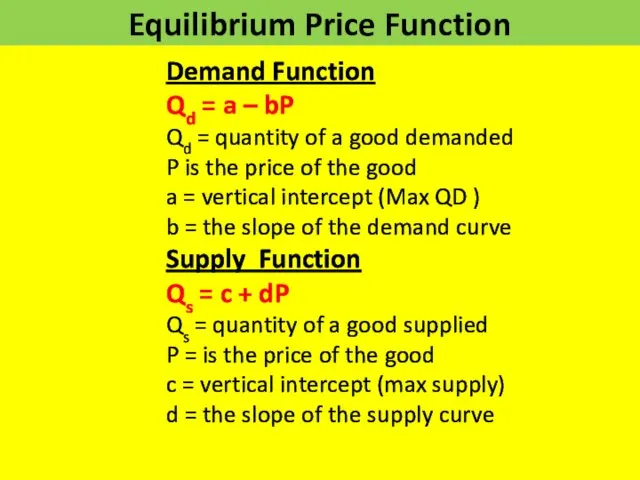
Equilibrium Price Function
Demand Function
Qd = a – bP
Qd =
Equilibrium Price Function
Demand Function
Qd = a – bP
Qd =
In Class Activity
01/11/2016
Sonali Sinha Roy
Consider the market for apple juice. In
In Class Activity
01/11/2016
Sonali Sinha Roy
Consider the market for apple juice. In

Recap of Today’s Lesson
01/11/2016
Sonali Sinha Roy
Recap of Today’s Lesson
01/11/2016
Sonali Sinha Roy
 Види договорів, що регулюють інвестиційний процес
 Оборотные средства предприятия
 Индивидуальное предложение для зарплатных клиентов
 Потребительское кредитование в России: состояние и пути его совершенствования на примере ПАО Сбербанка России
 География в купюрах
 Кассир – профессия для ответственных
 Налог на имущество физических лиц
 Фундаментальный анализ
 Международный валютный фонд (МВФ)
 Анализ и оценка имущественного состояния организации и источников его финансирования
 Возвратность кредита: проблемы и решения
 Учет и анализ доходов, расходов и финансовых результатов деятельности организации (на примере ОАО Башспирт)
 Финансовый контроль, формы и методы его проведения. Виды финансового контроля
 Налоговый калькулятор по расчету налоговой нагрузки
 Нематериальные необоротные активы
 Построение денежных потоков инвестиционного проекта по привлечению капитала
 Правовое регулирование финансового контроля
 Финансовый взлет
 Концептуальные магазины. Книга розничных мотиваций adidas Group
 Зарубежное накопительное страхование жизни
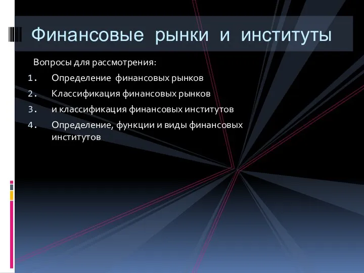 Финансовые рынки и институты
 Accounting and Financial Reporting
 Работа с программным обеспечением для роли Агент в рамках нового процесса выдачи POS-кредит/займов. АО ОТП БАНК
 Participation banks in the financial system of Turkey
 Методические приемы ревизии и контроля
 Фонд развития моногородов
 місцеві податки і збори. Інші податки
 Страхование финансовых рисков