- Normal Probability Distributions

Содержание
- 2. A density curve is the graph of a probability distribution of a continuous random variable. It
- 3. Because the total area under the density curve is equal to 1, there is a correspondence
- 4. Uniform Distribution (Definition) A continuous random variable has a uniform distribution if its values are spread
- 5. (Example) A power company provides electricity with voltage levels between 123.0 volts and 125.0 volts, and
- 6. Normal Probability Distribution Properties 1. A bell-shaped curve 2. The total area under the curve is
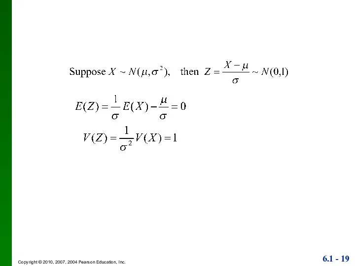
- 7. Standard Normal Distribution The standard normal distribution is a normal probability distribution with μ = 0
- 8. P(a P(Z > a) = probability that the z-score is greater than a. P(Z Finding probability
- 9. R for normal distribution dnorm(x, mean = 0, sd = 1) =density function, not P(X=0) pnorm(x,
- 10. Example Required area
- 11. Example z Shaded area is .4850 -2.17 0 Table 6.3 Area Under the Standard Normal Curve
- 12. Assume that the readings of a thermometer are normally distributed with the mean 0ºC and the
- 13. P(Z Example I P (Z The probability of randomly selecting a thermometer with a reading less
- 14. If one thermometer is randomly selected, find the probability that it reads, at the freezing point
- 15. A thermometer is randomly selected. Find the probability that it reads (at the freezing point of
- 16. Finding z Scores When Given Probabilities – Inverse problem Finding the 95th Percentile 5% or 0.05
- 17. Applications of Normal Distributions
- 18. Converting to a Standard Normal Distribution Conversion Formula :
- 20. Example Find P ( X Use Suppose X ~ N(μ , σ2), μ = 172, σ
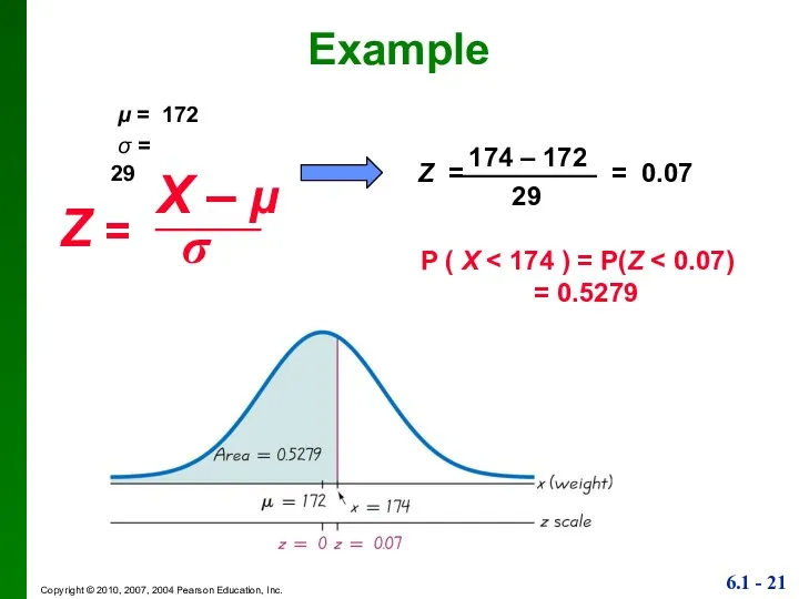
- 21. Example P ( X = 0.5279
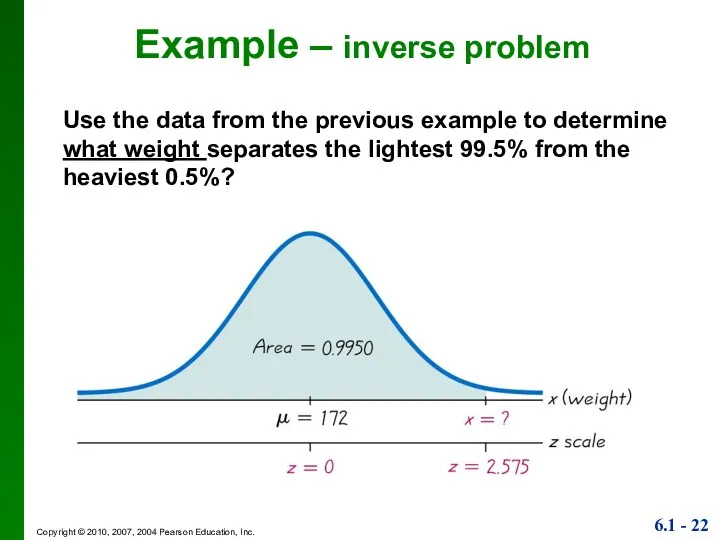
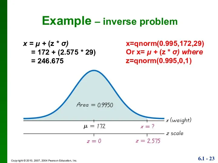
- 22. Example – inverse problem Use the data from the previous example to determine what weight separates
- 23. x = μ + (z * σ) = 172 + (2.575 * 29) = 246.675 Example
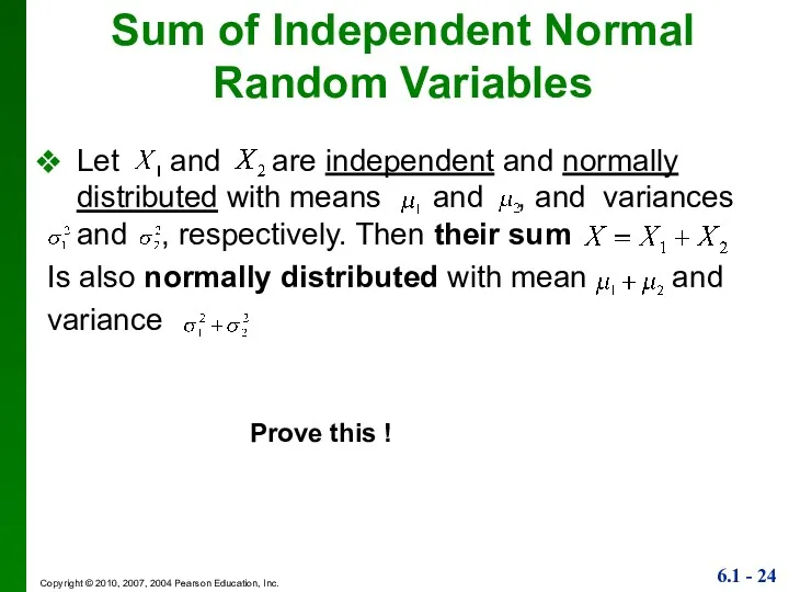
- 24. Sum of Independent Normal Random Variables Let and are independent and normally distributed with means and
- 25. The Central Limit Theorem
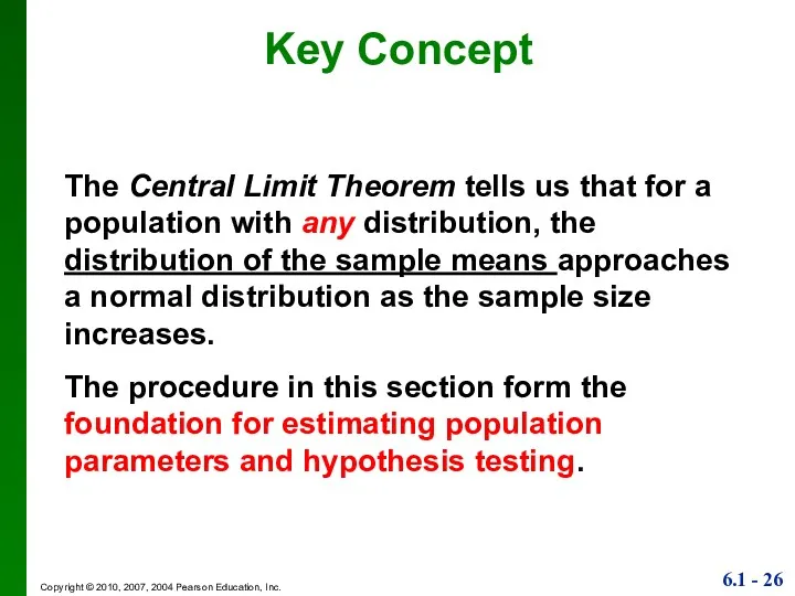
- 26. Key Concept The Central Limit Theorem tells us that for a population with any distribution, the
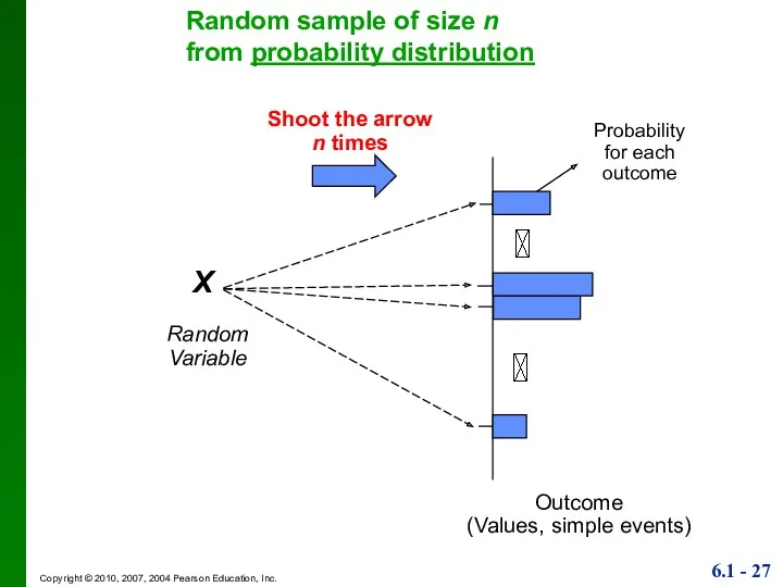
- 27. X Random Variable Shoot the arrow n times Outcome (Values, simple events) Probability for each outcome
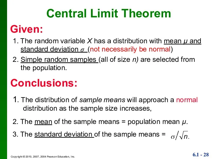
- 28. Central Limit Theorem 1. The random variable X has a distribution with mean µ and standard
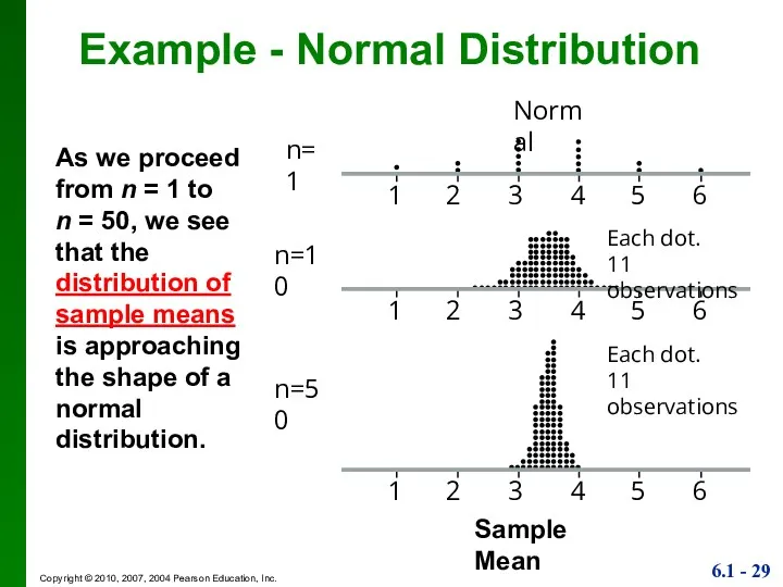
- 29. Example - Normal Distribution As we proceed from n = 1 to n = 50, we
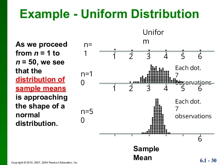
- 30. Example - Uniform Distribution As we proceed from n = 1 to n = 50, we
- 31. Example - U-Shaped Distribution As we proceed from n = 1 to n = 50, we
- 32. Notation the mean of the sample mean the standard deviation of sample mean Show them !
- 33. Informal: Whatever the population, the distribution of is normal with mean and standard deviation when n
- 34. Practical Rules Commonly Used (Case 1) The original population is normally distributed. For any sample size
- 35. Assume the population of weights of men is normally distributed with a mean of 172 lb
- 36. a) Find the probability that if an individual man is randomly selected, his weight is greater
- 37. b) Find the probability that 20 randomly selected men will have a mean weight that is
- 38. Assume the population of weights of men has a mean of 172 lb and a standard
- 39. Normal as Approximation to Binomial
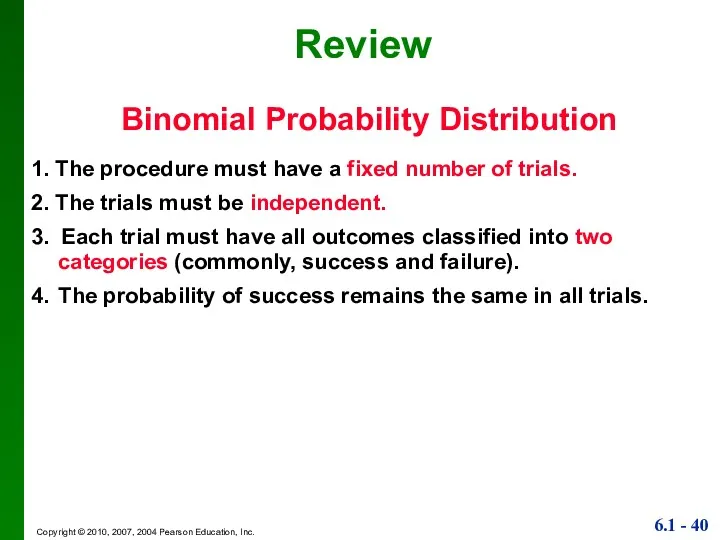
- 40. Review Binomial Probability Distribution 1. The procedure must have a fixed number of trials. 2. The
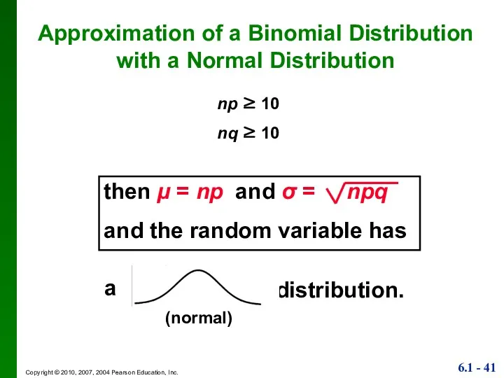
- 41. Approximation of a Binomial Distribution with a Normal Distribution np ≥ 10 nq ≥ 10
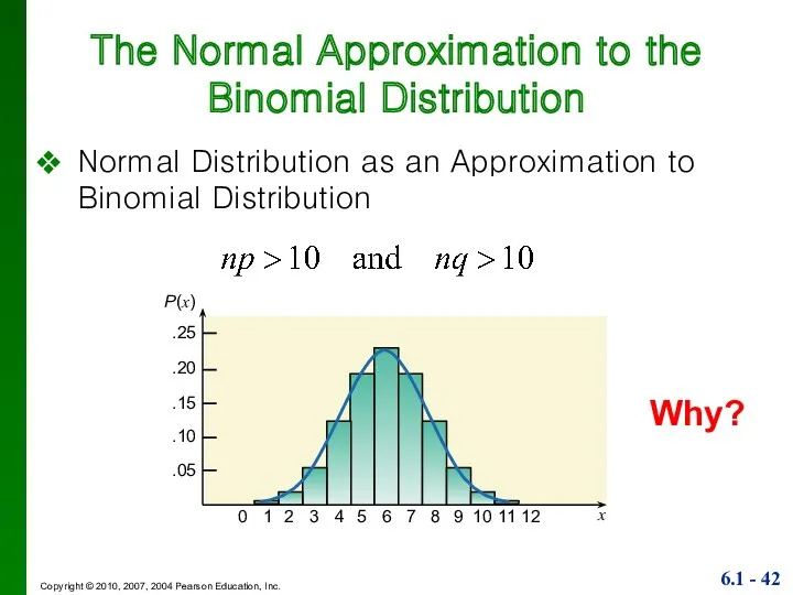
- 42. The Normal Approximation to the Binomial Distribution Normal Distribution as an Approximation to Binomial Distribution .25
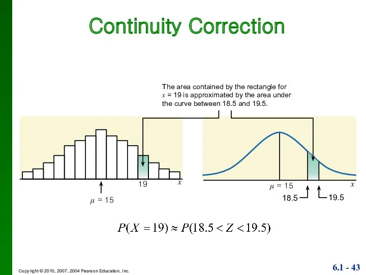
- 43. Continuity Correction x 18.5 19 μ = 15 x The area contained by the rectangle for
- 44. Procedure for Using a Normal Distribution to Approximate a Binomial Distribution 1. Check that np ≥
- 45. 4. Draw a normal distribution centered about μ, then draw a vertical strip area centered over
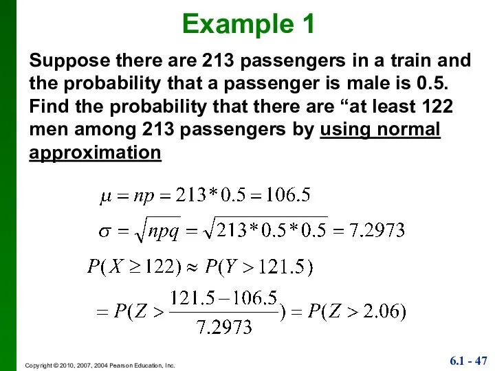
- 46. Suppose there are 213 passengers in a train and the probability that a passenger is male
- 47. Suppose there are 213 passengers in a train and the probability that a passenger is male
- 49. Скачать презентацию
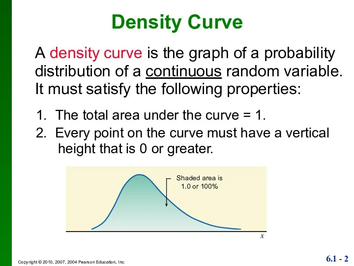
A density curve is the graph of a probability distribution of
A density curve is the graph of a probability distribution of
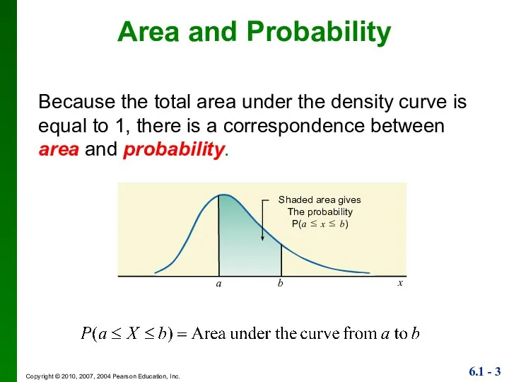
Because the total area under the density curve is equal to
Because the total area under the density curve is equal to
Uniform Distribution
(Definition) A continuous random variable has a uniform distribution if
Uniform Distribution
(Definition) A continuous random variable has a uniform distribution if
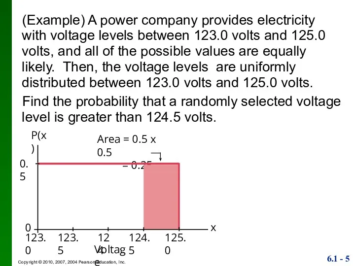
(Example) A power company provides electricity with voltage levels between 123.0
(Example) A power company provides electricity with voltage levels between 123.0
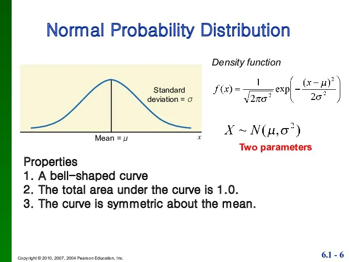
Normal Probability Distribution
Properties
1. A bell-shaped curve
2. The total area under the
Normal Probability Distribution
Properties
1. A bell-shaped curve
2. The total area under the
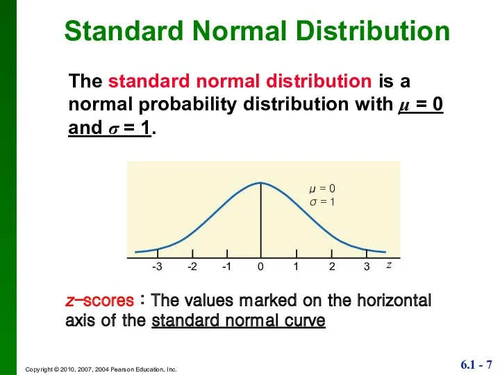
Standard Normal Distribution
The standard normal distribution is a normal probability distribution
Standard Normal Distribution
The standard normal distribution is a normal probability distribution
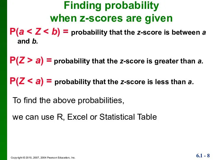
P(a < Z < b) = probability that the z-score is
P(a < Z < b) = probability that the z-score is
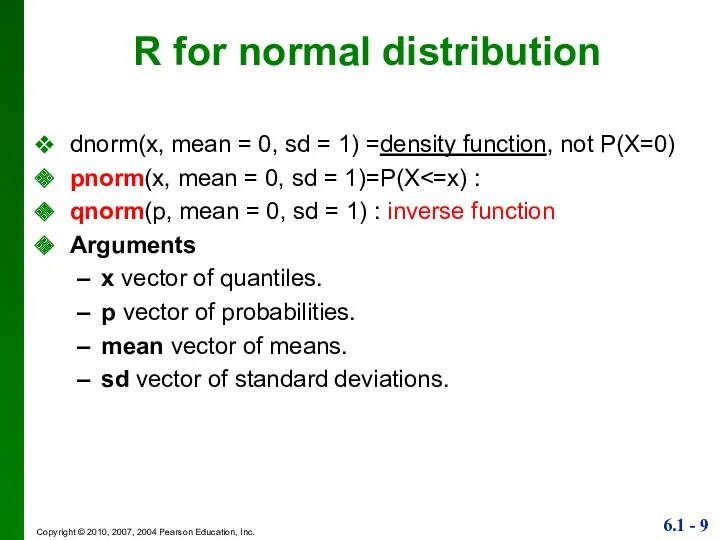
R for normal distribution
dnorm(x, mean = 0, sd = 1) =density
R for normal distribution
dnorm(x, mean = 0, sd = 1) =density
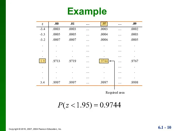
Example
Required area
Example
Required area
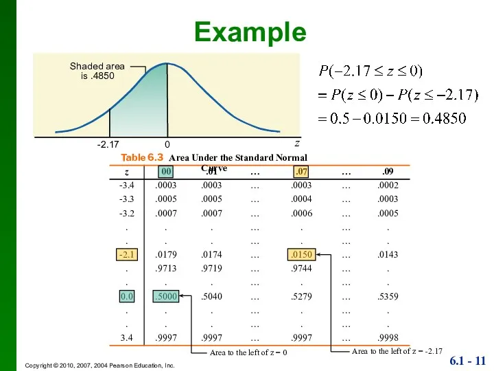
Example
z
Shaded area
is .4850
-2.17
0
Table 6.3 Area Under the Standard Normal Curve
Area to
Example
z
Shaded area
is .4850
-2.17
0
Table 6.3 Area Under the Standard Normal Curve
Area to
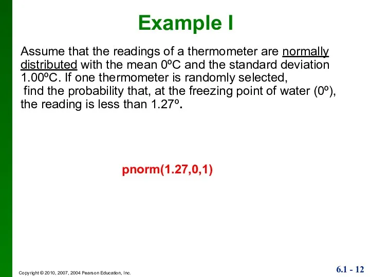
Assume that the readings of a thermometer are normally distributed with
Assume that the readings of a thermometer are normally distributed with
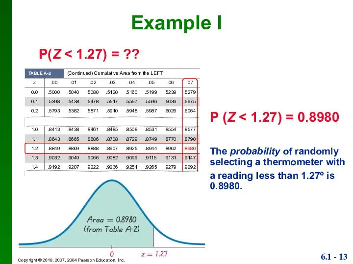
P(Z < 1.27) = ??
Example I
P (Z < 1.27) = 0.8980
The
P(Z < 1.27) = ??
Example I
P (Z < 1.27) = 0.8980
The
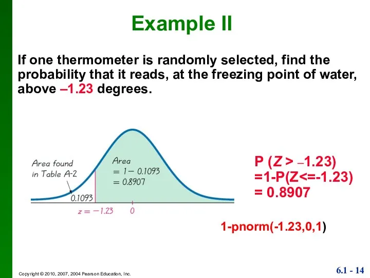
If one thermometer is randomly selected, find the probability that it
If one thermometer is randomly selected, find the probability that it
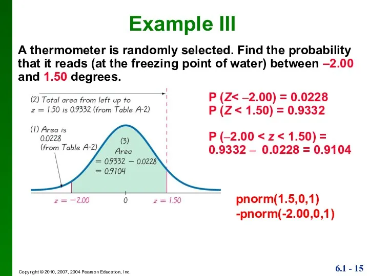
A thermometer is randomly selected. Find the probability that it reads
A thermometer is randomly selected. Find the probability that it reads
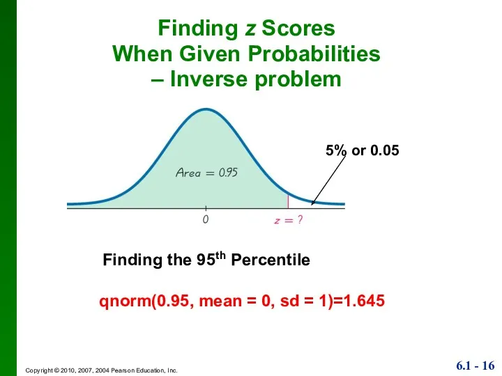
Finding z Scores
When Given Probabilities
– Inverse problem
Finding the 95th
Finding z Scores
When Given Probabilities
– Inverse problem
Finding the 95th

Applications of Normal Distributions
Applications of Normal Distributions
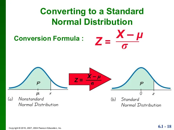
Converting to a Standard
Normal Distribution
Conversion Formula :
Converting to a Standard
Normal Distribution
Conversion Formula :
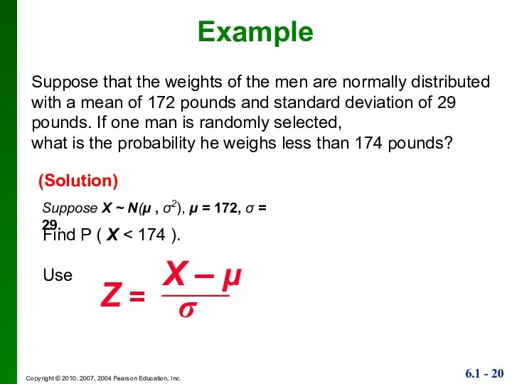
Example
Find P ( X < 174 ).
Use
Suppose X ~ N(μ
Example
Find P ( X < 174 ).
Use
Suppose X ~ N(μ
Example
P ( X < 174 ) = P(Z < 0.07)
=
Example
P ( X < 174 ) = P(Z < 0.07)
=
Example – inverse problem
Use the data from the previous example to
Example – inverse problem
Use the data from the previous example to
x = μ + (z * σ)
= 172 + (2.575
x = μ + (z * σ)
= 172 + (2.575
Sum of Independent Normal Random Variables
Let and are independent and normally
Sum of Independent Normal Random Variables
Let and are independent and normally
The Central Limit Theorem
The Central Limit Theorem
Key Concept
The Central Limit Theorem tells us that for a population
Key Concept
The Central Limit Theorem tells us that for a population
X
Random
Variable
Shoot the arrow
n times
Outcome
(Values, simple events)
Probability
for each
outcome
Random sample
X
Random
Variable
Shoot the arrow
n times
Outcome
(Values, simple events)
Probability
for each
outcome
Random sample
Central Limit Theorem
1. The random variable X has a distribution
Central Limit Theorem
1. The random variable X has a distribution
Example - Normal Distribution
As we proceed from n = 1 to
n
Example - Normal Distribution
As we proceed from n = 1 to n
Example - Uniform Distribution
As we proceed from n = 1 to
n
Example - Uniform Distribution
As we proceed from n = 1 to n
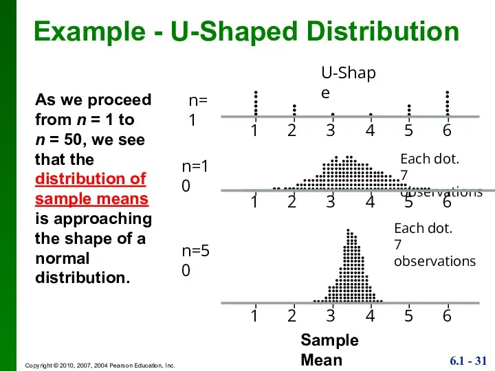
Example - U-Shaped Distribution
As we proceed from n = 1 to
n
Example - U-Shaped Distribution
As we proceed from n = 1 to n
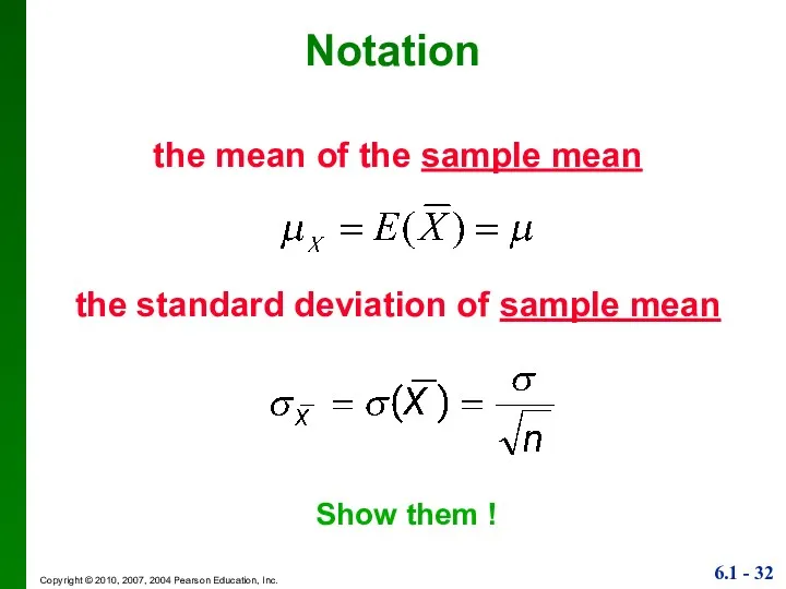
Notation
the mean of the sample mean
the standard deviation of sample mean
Show
Notation
the mean of the sample mean
the standard deviation of sample mean
Show
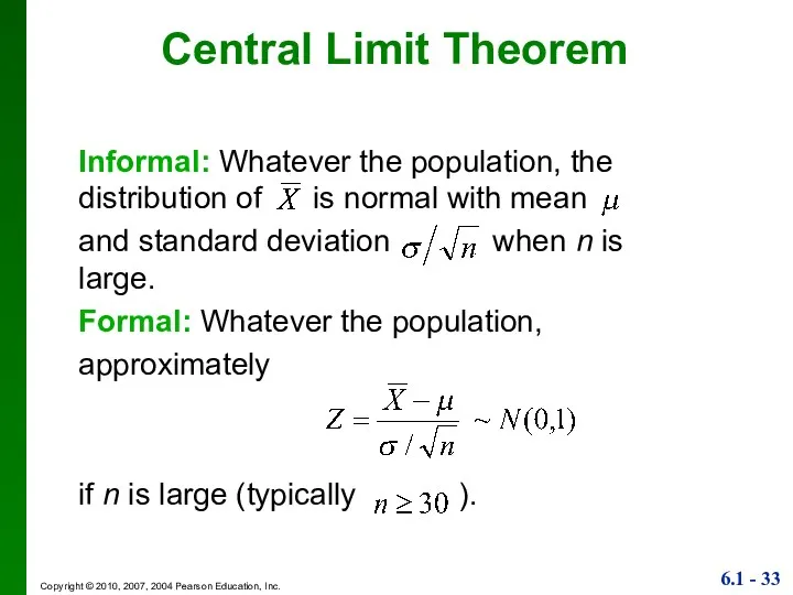
Informal: Whatever the population, the distribution of is normal with mean
and
Informal: Whatever the population, the distribution of is normal with mean
and
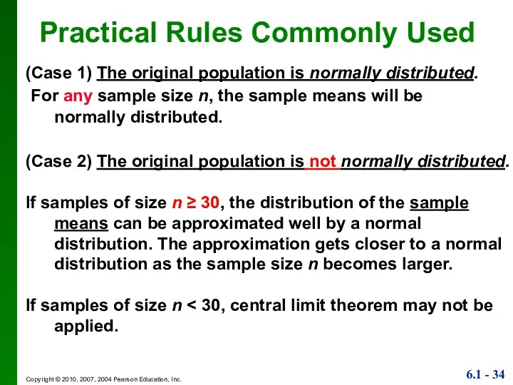
Practical Rules Commonly Used
(Case 1) The original population is normally distributed.
Practical Rules Commonly Used
(Case 1) The original population is normally distributed.
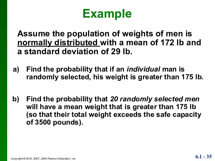
Assume the population of weights of men is normally distributed with
Assume the population of weights of men is normally distributed with
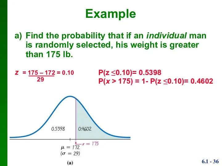
a) Find the probability that if an individual man is randomly selected,
a) Find the probability that if an individual man is randomly selected,
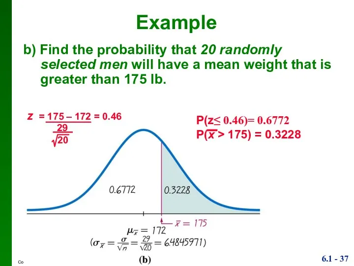
b) Find the probability that 20 randomly selected men will have
b) Find the probability that 20 randomly selected men will have
Assume the population of weights of men has a mean of
Assume the population of weights of men has a mean of
Normal as Approximation to Binomial
Normal as Approximation to Binomial
Review
Binomial Probability Distribution
1. The procedure must have a fixed number
Review
Binomial Probability Distribution
1. The procedure must have a fixed number
Approximation of a Binomial Distribution
with a Normal Distribution
np ≥ 10
nq ≥
Approximation of a Binomial Distribution
with a Normal Distribution
np ≥ 10
nq ≥
The Normal Approximation to the Binomial Distribution
Normal Distribution as an Approximation
The Normal Approximation to the Binomial Distribution
Normal Distribution as an Approximation
Continuity Correction
x
18.5
19
μ = 15
x
The area contained by the rectangle for
x =
Continuity Correction
x
18.5
19
μ = 15
x
The area contained by the rectangle for
x =
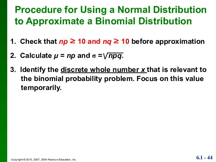
Procedure for Using a Normal Distribution to Approximate a Binomial Distribution
1.
Procedure for Using a Normal Distribution to Approximate a Binomial Distribution
1.
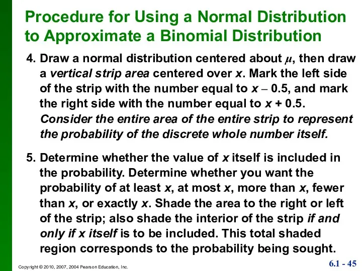
4. Draw a normal distribution centered about μ, then draw a vertical
4. Draw a normal distribution centered about μ, then draw a vertical
Suppose there are 213 passengers in a train and the probability
Suppose there are 213 passengers in a train and the probability
Suppose there are 213 passengers in a train and the probability
Suppose there are 213 passengers in a train and the probability
 Линейная функция. Алгебра, 7 класс
 Десятичные дроби. Задания для устного счета
 Решение линейных уравнений с одной переменной
 Параллелепипед и куб
 Предел функции. Непрерывность функции. Точки разрыва
 Решение задач с процентами: нахождение числа по процентам. 5 класс
 Алгебраическая сумма и её свойства
 Красота в математике или применение векторов к доказательству стереометрических теорем
 Решение задач на применение аксиом стереометрии и их следствий
 Презентация к уроку Прибавление чисел 7, 8. 9
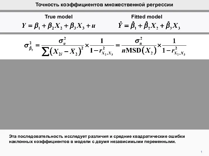 Точность коэффициентов множественной регрессии
 Регрессионный анализ
 Случаи сложения вида +4
 КВН по математике
 Десятичные дроби. Повторение. Действия с десятичными дробями
 ПРЕЗЕНТАЦИЯ ОБЪЕМ
 Симметрия в химии
 Сложение и вычитание чисел
 Сходимость знакоположительных рядов
 Матриці, дії з матрицями. Визначники, їх властивості
 Формулирование факторов для использования их в статистической модели
 Умножение круглых многозначных чисел
 Подготовка к ЕГЭ. Задача В8
 Длина окружности. 6 класс:
 Готовимся к ЕГЭ: задачи на проценты
 Сложение и вычитание положительных и отрицательных чисел. 6 класс
 Среднее арифметическое
 Решение задач. 1 класс