- Mathematics in Finance

Содержание
- 2. Contents American options The obstacle problem Discretisation methods Matlab results Recent insights and developments
- 3. 1. American options American options can be executed any time before expiry date, as opposed to
- 4. Bounds for prices (no dividends) For American options: For European options: Reminder: put-call parity
- 5. Why is ? Suppose we exercise the American call at time t Then we obtain St-K
- 6. What about put options? For put options, a similar reasoning shows that it may be advantageous
- 7. American options are more expensive than European options Comparison European-American options
- 8. An optimum time for exercising…. (1) Statement: There is Sf such that premature exercising is worthwhile
- 9. An optimum time for exercising…. (2) The value Sf depends on time, and it is termed
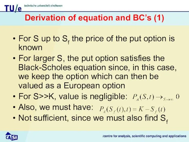
- 10. Derivation of equation and BC’s (1) For S up to Sf the price of the put
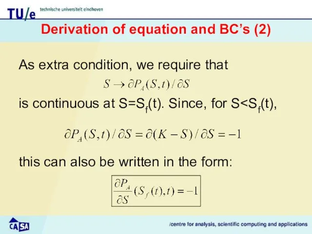
- 11. Derivation of equation and BC’s (2) As extra condition, we require that is continuous at S=Sf(t).
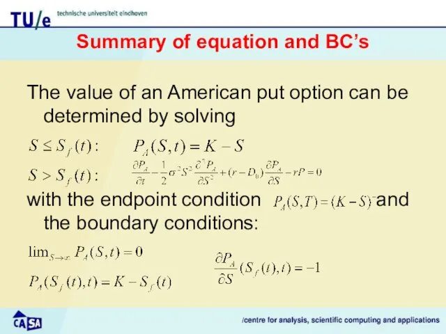
- 12. Summary of equation and BC’s The value of an American put option can be determined by
- 13. How to solve? Free boundary problems can be rewritten in the form of a linear complimentarity
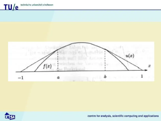
- 14. 2. The obstacle problem Consider a rope: fixed at endpoints –1 and 1 to be spanned
- 16. The linear complimentarity problem We rewrite the above properties as follows: and hence: So we can
- 17. Formulation without second derivatives Lemma 1: Define Then finding a solution of the LCP is equivalent
- 18. What about minimum length? The latter is again equal to the following problem: Find with the
- 19. Summarizing so far The obstacle problem can be formulated As a free boundary problem As a
- 20. 3. Discretisation methods
- 21. Finite difference method (1) If we choose to solve the LCP, we can use the FD
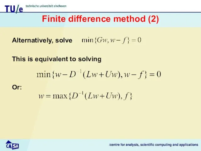
- 22. Finite difference method (2) Alternatively, solve This is equivalent to solving Or:
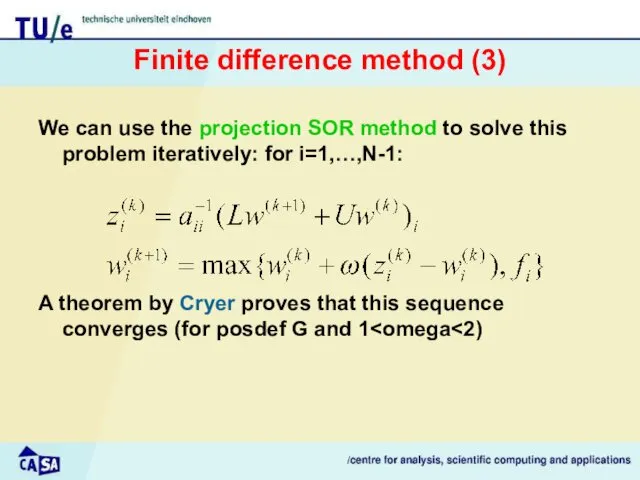
- 23. Finite difference method (3) We can use the projection SOR method to solve this problem iteratively:
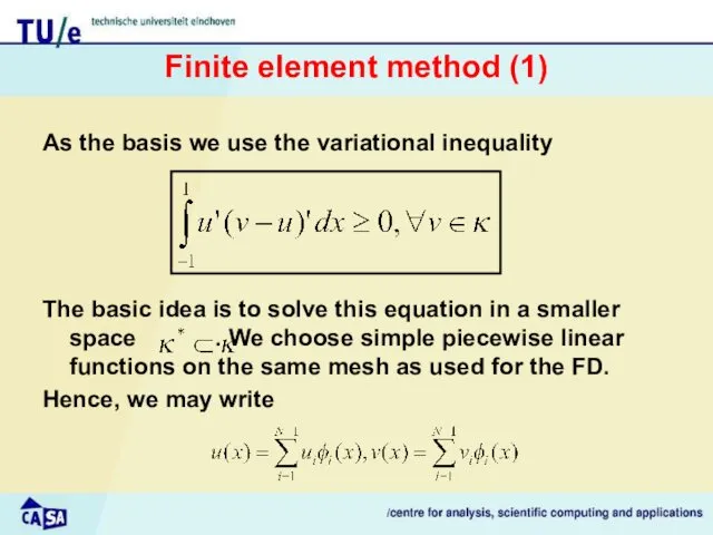
- 24. Finite element method (1) As the basis we use the variational inequality The basic idea is
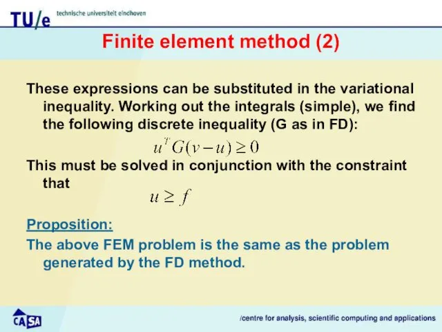
- 25. Finite element method (2) These expressions can be substituted in the variational inequality. Working out the
- 26. Summary: comparison of FD and FEM Finite difference method: Finite element method:
- 27. 4. Implementation in Matlab
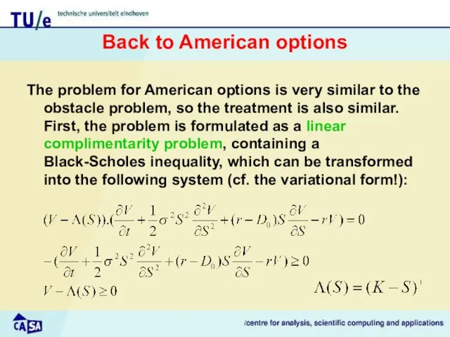
- 28. Back to American options The problem for American options is very similar to the obstacle problem,
- 29. Result of Matlab calculation using projection SOR K=100, r=0.1, sigma=0.4, T=1
- 30. Number of iterations in projection SOR method Depending on the overrelaxation parameter omega
- 31. 5. Recent insights and developments
- 32. Historical account First widely-used methods using FD by Brennan and Schwartz (1977) and Cox et al.
- 33. Recent work (1) Some people concentrate on Monte Carlo methods to evaluate the discounted integrals of
- 35. Скачать презентацию
Contents
American options
The obstacle problem
Discretisation methods
Matlab results
Recent insights and developments
Contents
American options
The obstacle problem
Discretisation methods
Matlab results
Recent insights and developments
1. American options
American options can be executed any time before
1. American options
American options can be executed any time before
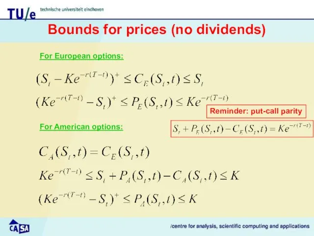
Bounds for prices (no dividends)
For American options:
For European options:
Reminder: put-call parity
Bounds for prices (no dividends)
For American options:
For European options:
Reminder: put-call parity
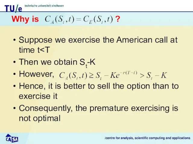
Why is ?
Suppose we exercise the American call at time
Why is ?
Suppose we exercise the American call at time
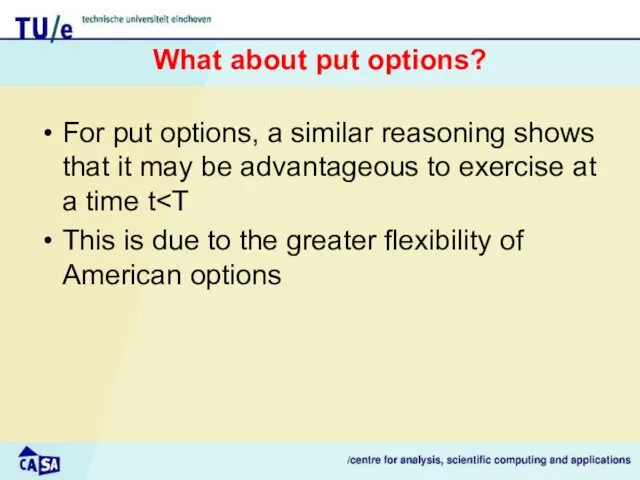
What about put options?
For put options, a similar reasoning shows that
What about put options?
For put options, a similar reasoning shows that
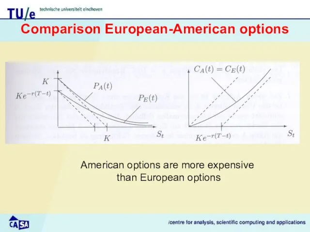
American options are more expensive
than European options
Comparison European-American options
American options are more expensive
than European options
Comparison European-American options
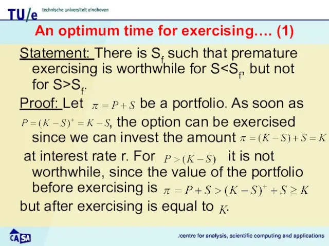
An optimum time for exercising…. (1)
Statement: There is Sf such that
An optimum time for exercising…. (1)
Statement: There is Sf such that
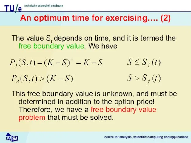
An optimum time for exercising…. (2)
The value Sf depends on time,
An optimum time for exercising…. (2)
The value Sf depends on time,
Derivation of equation and BC’s (1)
For S up to Sf the
Derivation of equation and BC’s (1)
For S up to Sf the
Derivation of equation and BC’s (2)
As extra condition, we require that
Derivation of equation and BC’s (2)
As extra condition, we require that
Summary of equation and BC’s
The value of an American put option
Summary of equation and BC’s
The value of an American put option
How to solve?
Free boundary problems can be rewritten in the form
How to solve?
Free boundary problems can be rewritten in the form
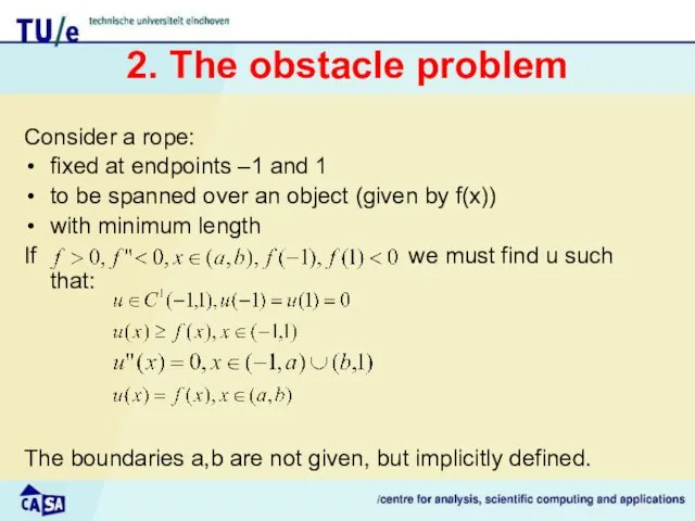
2. The obstacle problem
Consider a rope:
fixed at endpoints –1 and 1
to
2. The obstacle problem
Consider a rope:
fixed at endpoints –1 and 1
to
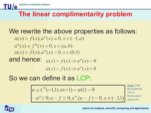
The linear complimentarity problem
We rewrite the above properties as follows:
and hence:
So
The linear complimentarity problem
We rewrite the above properties as follows:
and hence:
So
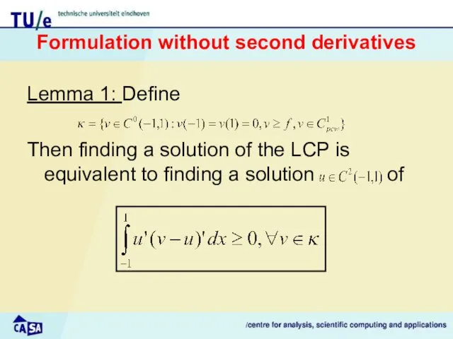
Formulation without second derivatives
Lemma 1: Define
Then finding a solution of the
Formulation without second derivatives
Lemma 1: Define
Then finding a solution of the
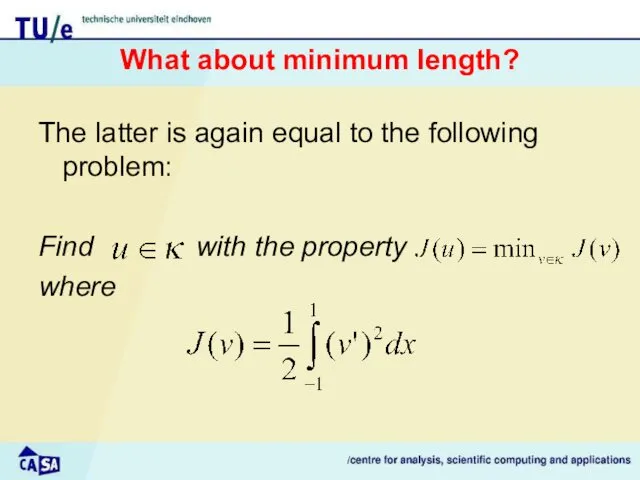
What about minimum length?
The latter is again equal to the following
What about minimum length?
The latter is again equal to the following
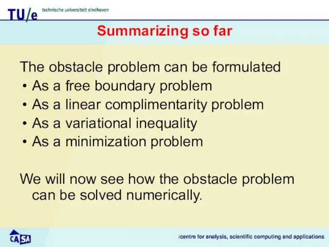
Summarizing so far
The obstacle problem can be formulated
As a free boundary
Summarizing so far
The obstacle problem can be formulated
As a free boundary
3. Discretisation methods
3. Discretisation methods
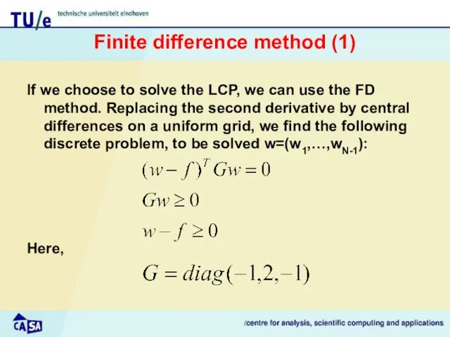
Finite difference method (1)
If we choose to solve the LCP, we
Finite difference method (1)
If we choose to solve the LCP, we
Finite difference method (2)
Alternatively, solve
This is equivalent to solving
Or:
Finite difference method (2)
Alternatively, solve
This is equivalent to solving
Or:
Finite difference method (3)
We can use the projection SOR method to
Finite difference method (3)
We can use the projection SOR method to
Finite element method (1)
As the basis we use the variational inequality
The
Finite element method (1)
As the basis we use the variational inequality
The
Finite element method (2)
These expressions can be substituted in the variational
Finite element method (2)
These expressions can be substituted in the variational
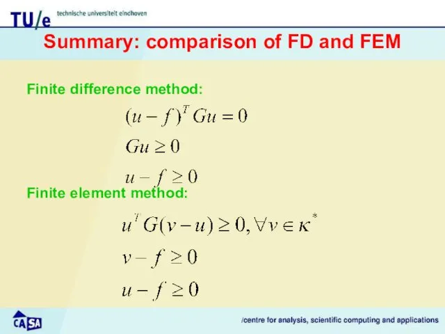
Summary: comparison of FD and FEM
Finite difference method:
Finite element method:
Summary: comparison of FD and FEM
Finite difference method:
Finite element method:
4. Implementation in Matlab
4. Implementation in Matlab
Back to American options
The problem for American options is very similar
Back to American options
The problem for American options is very similar
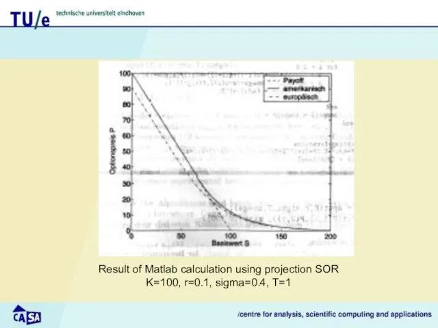
Result of Matlab calculation using projection SOR
K=100, r=0.1, sigma=0.4, T=1
Result of Matlab calculation using projection SOR
K=100, r=0.1, sigma=0.4, T=1
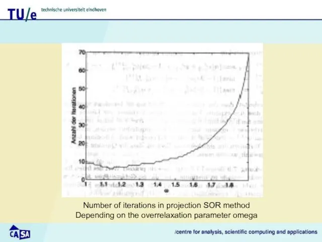
Number of iterations in projection SOR method
Depending on the overrelaxation parameter
Number of iterations in projection SOR method
Depending on the overrelaxation parameter

5. Recent insights and developments
5. Recent insights and developments
Historical account
First widely-used methods using FD by Brennan and Schwartz (1977)
Historical account
First widely-used methods using FD by Brennan and Schwartz (1977)
Recent work (1)
Some people concentrate on Monte Carlo methods to evaluate
Recent work (1)
Some people concentrate on Monte Carlo methods to evaluate
 The theory of exchange rate determination
 Что такое деньги
 Собственные средства (капитал) банка
 Изменения в бухгалтерском учете учреждений бюджетной сферы вступающие в силу с 2023 года
 Зменения законодательства по вопросам персонифицированного учета
 Topic 1. Introduction to Finance
 Студенческий совет факультета ПМ-ПУ. Информационное собрание на тему: Повышенная академическая стипендия
 Зарплатный проект
 Основы аудита
 Инвестиционная программа МУП Яргорэнергосбыт г. Ярославля по повышению качества горячего водоснабжения
 Учет расчетных операций
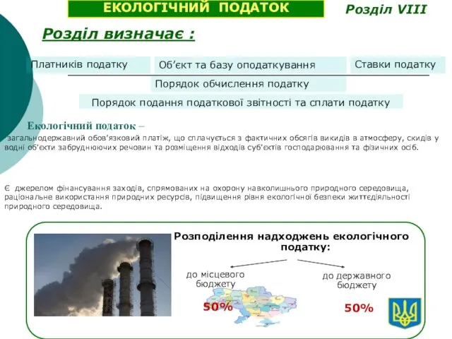 Екологічний податок
 РКМЦ по Самарской области
 Трейдинг как привилегия
 Портфели ценных бумаг
 Фандрайзинг с картинками
 Анализ и оценка платежеспособности и ликвидности предприятия на примере ООО СМК Аудит
 Спортивный плюс. СК Благосостояние
 МСА 520 Аналитические процедуры
 Финансирование бизнеса
 Предоставление мер социальной поддержки по оплате жилого помещения и коммунальных услуг работающим гражданам указанных в статье
 Спрос на деньги. Денежно-кредитная политика
 Место и роль платежных карт в системе безналичных расчетов
 Корпоративные финансы. Тема 1. Экономическая сущность и особенности корпоративных финансов
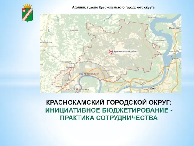 Результативность участия Краснокамского городского округа в конкурсе проектов инициативного бюджетирования
 Учет запасов. Оценка запасов. Учет поступления и выбытия запасов
 Финансы домашних хозяйств
 Нематериальные активы