Методы исследования взаимодействий с участием белков (Co-IP, equilibrium microdialysis, ITC, MST, SPR, BLI, QСM) презентация
- Методы исследования взаимодействий с участием белков (Co-IP, equilibrium microdialysis, ITC, MST, SPR, BLI, QСM)

Содержание
- 2. Protein-protein interactions (PPIs) >80% of proteins function via interaction with other proteins (PMID: 17640003) For each
- 3. Interactions of proteins control the life of the cell
- 4. Interactions of proteins control the life of the cell … cell biochemistry would appear to be
- 5. Types of PPIs
- 6. Types of PPIs Homologous interactions: • The same proteins • Oligomers • Coiled-coil • Amyloids Heterologous
- 8. Types of PPIs Qualitative methods: • Co-immunoprecipitation (Co-IP) • Pull-down Quantitative methods: • Isothermal titration calorimetry
- 9. Detecting PPI: co-immunoprecipitation (Co-IP)
- 10. Reciprocal Co-IP in investigation of 14-3-3 interacting proteins Direct Immunoprecipitation of 14-3-3 and detection of bound
- 11. Tandem affinity purification (TAP)
- 12. M + L ML M is free macromolecule L is free ligand ML is complex Lo
- 13. Simple binding A+B ↔ AB quadratic equation https://www.symbolab.com/solver/equation-calculator/%5Cleft(100-x%5Cright)%5Ccdot%5Cleft(10-x%5Cright)-15%5Ccdot%20x%3D0 Online quadratic equation solver: (just put your numbers
- 14. Simple binding A+B ↔ AB quadratic equation https://www.symbolab.com/solver/equation-calculator/%5Cleft(100-x%5Cright)%5Ccdot%5Cleft(10-x%5Cright)-15%5Ccdot%20x%3D0 Online quadratic equation solver: (just put your numbers
- 15. Dimerization process M + M M2 or D Kd = [M][M]/[D] = [M]2/[D] [Mo] = [M]
- 16. For a reversible process, one can assess thermodynamics of binding Kd = 1/Keq ΔGo = -
- 17. For a reversible process, one can assess thermodynamics of binding Kd = 1/Keq ΔGo = -
- 18. ΔGo = R T ln KD @ 20 °C
- 19. At equilibrium, both forward and reverse reaction rates are equal Kd = 1/Keq kon koff Von
- 20. Thermodynamics of interaction Gibbs free energy Enthalpy Entropy R T ln KD =
- 21. Binding affinity range http://www.bindingdb.org/bind/index.jsp 1,772,210 binding data : http://www.pdbbind-cn.org
- 22. Methods to study PPI (and other interactions!) Equilibrium microdialysis (EMD) Fluorescence polarization (FP) Isothermal titration calorimetry
- 23. Equilibrium microdialysis (EMD) Two chambers of equal volume facing each other Semipermeable membrane separates the two
- 24. Equilibrium microdialysis (EMD) L total is known L free is measured -> L bound is calculated
- 25. Equilibrium microdialysis (EMD) KD = [M] * [L] [ML] M + L ML Fast Easy Inexpensive
- 26. Equilibrium microdialysis (EMD) DOI: 10.1021/acschemneuro.8b00111 Thioflavin T (ThT) binding to acetylcholinesterase (AChE) AChE
- 27. Fluorescence polarization (FP) The degree of polarization is associated with the size of the particle bearing
- 28. Fluorescence polarization (P) or anisotropy (r): no nominal dependence on dye concentration P has physically possible
- 29. Fluorescence polarization and molecular size η = solvent viscosity, T = temperature, R = gas constant
- 30. FP features Great tool to study interactions Small sample consumption Low limit of detection Rapid response
- 31. FP is very good for high-throughput studies DOI: 10.1002/1873-3468.13017
- 32. Isothermal titration calorimetry (ITC) Sangho Lee (c) https://www.youtube.com/watch?v=o_IpWcWKNXI
- 33. Isothermal titration calorimetry (ITC) Sangho Lee (c)
- 34. ITC experiment • Exothermic reaction (common for PPI) • The sample cell becomes warmer than the
- 35. ITC thermogram stoichiometry 1/KD C of macromolecule in the cell Determined in the experiment Is calculated
- 36. Small-molecule stabilizer of protein-peptide interaction
- 37. ITC pros and cons Advantages: Ability to determine thermodynamic binding parameters (i.e. stoichiometry, association constant, and
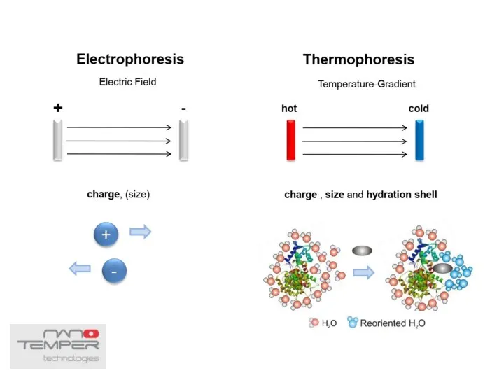
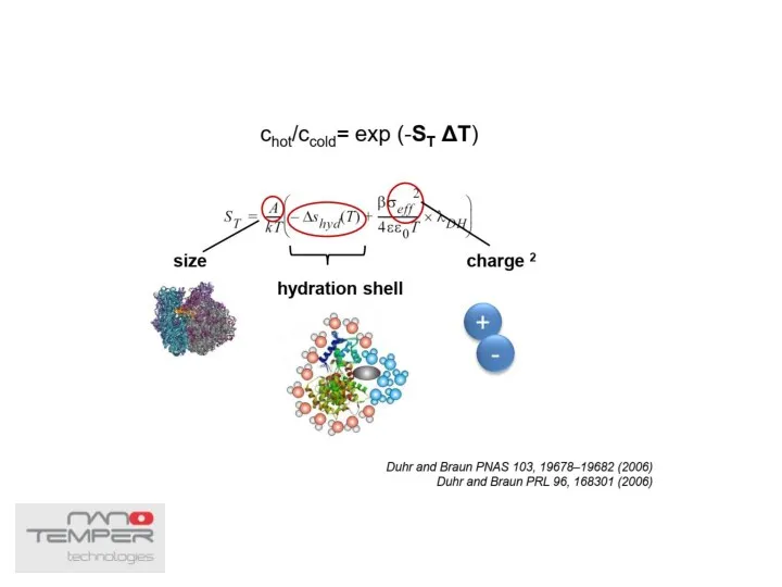
- 38. Thermophoresis The movement of molecules in a temperature gradient
- 41. Phases of MST experiment
- 42. Typical MST binding curve
- 43. Microscale thermophoresis (MST) https://www.youtube.com/watch?v=4U-0lyHQ0wg https://www.youtube.com/watch?v=rCot5Nfi_Og
- 44. MST data examples
- 46. MST pros and cons Advantages: Small sample size Immobilization free Minimal contamination of the sample (method
- 47. Surface plasmon resonance (SPR)
- 48. Reflection and refraction at different angles
- 49. Surface plasmon resonance (SPR) Patching, Biochim. Biophys. Acta (2014) https://youtu.be/o8d46ueAwXI https://www.youtube.com/watch?v=oUwuCymvyKc https://www.youtube.com/watch?v=sM-VI3alvAI
- 50. SPR sensorgram
- 51. Chips Biacore
- 52. Why is kinetic analysis important?
- 53. Practical considerations Use several concentrations (ideally, 10 times below till 10 times above KD) Accurate protein
- 54. Data analysis by simultaneous fitting of all curves using a binding model Biacore
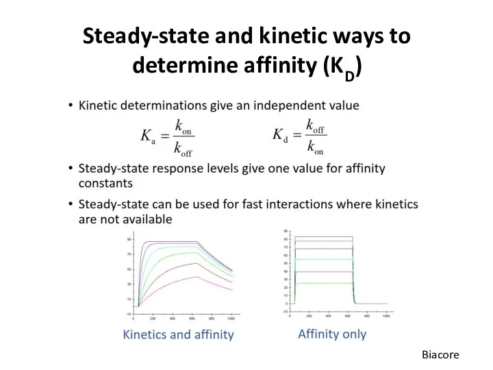
- 55. Steady-state and kinetic ways to determine affinity (KD) Biacore
- 56. Steady-state and kinetic ways to determine affinity (KD) Biacore
- 57. SPR pros and cons Advantages: Label-free detection Real-time data (i.e. quantitative binding affinities, kinetics and thermodynamics)
- 58. Biolayer interferometry (BLI) ForteBio; Citartan et al. Analyst (2013) https://www.moleculardevices.com/applications/biologics/bli-technology#gref
- 59. Instruments 8 channels 1 channel
- 60. Instruments 8 channels 1 channel
- 61. BLI sensorgrams Key Benefits of BLI Label-free detection Real-time results Simple and fast Improves efficiency Crude
- 62. BLI pros and cons Advantages: Label-free detection Real-time data No reference channel required Crude sample compatibility
- 63. ITC vs SPR and BLI comparison
- 64. Quartz crystal microbalance (QCM) High frequent oscillations of the quartz crystal (5-10 MHz) with the Au
- 65. Microfluidics delivers the sample and the deposited mass fraction is measured https://www.youtube.com/watch?v=xDKOUpSR3EQ
- 67. Скачать презентацию
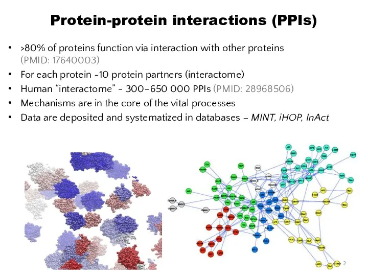
Protein-protein interactions (PPIs)
>80% of proteins function via interaction with other proteins
Protein-protein interactions (PPIs)
>80% of proteins function via interaction with other proteins
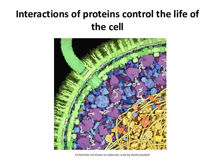
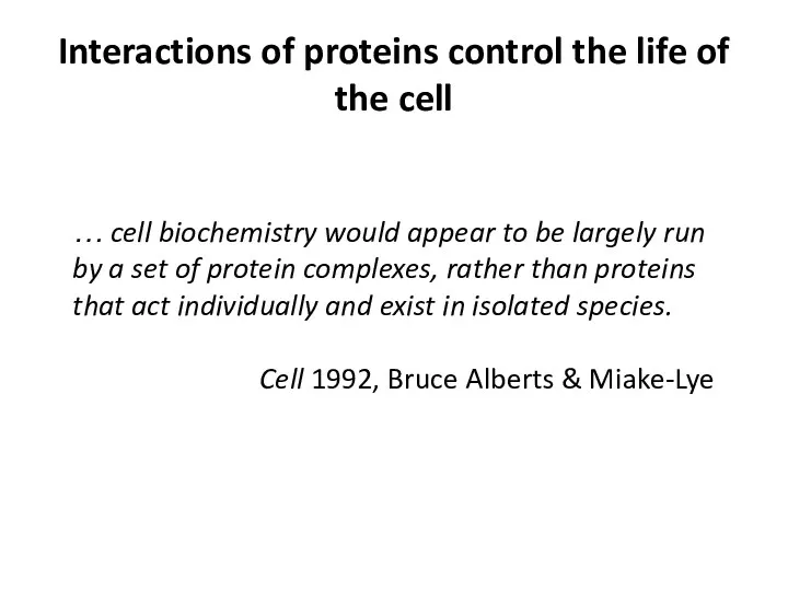
Interactions of proteins control the life of the cell
Interactions of proteins control the life of the cell
Interactions of proteins control the life of the cell
… cell biochemistry
Interactions of proteins control the life of the cell
… cell biochemistry
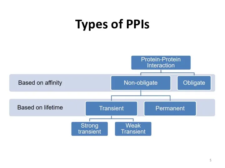
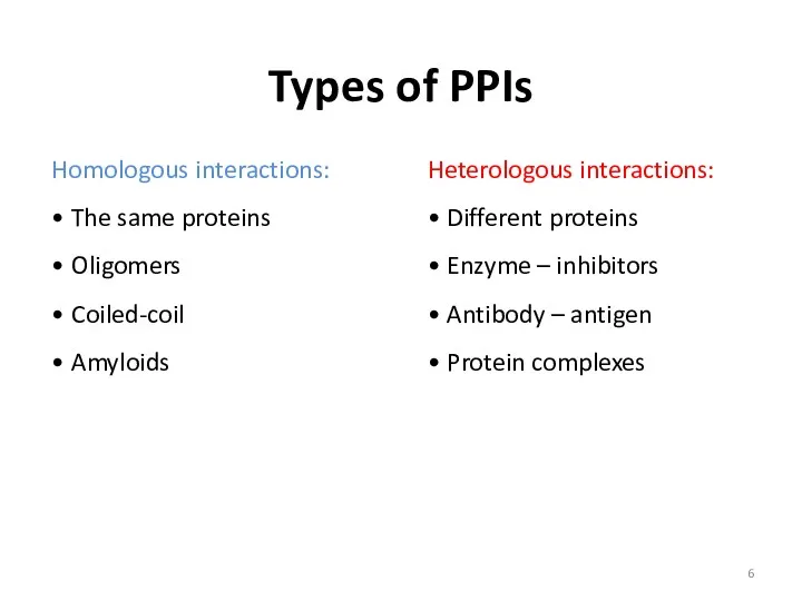
Types of PPIs
Types of PPIs
Types of PPIs
Homologous interactions:
• The same proteins
• Oligomers
• Coiled-coil
• Amyloids
Heterologous interactions:
•
Types of PPIs
Homologous interactions:
• The same proteins
• Oligomers
• Coiled-coil
• Amyloids
Heterologous interactions: •
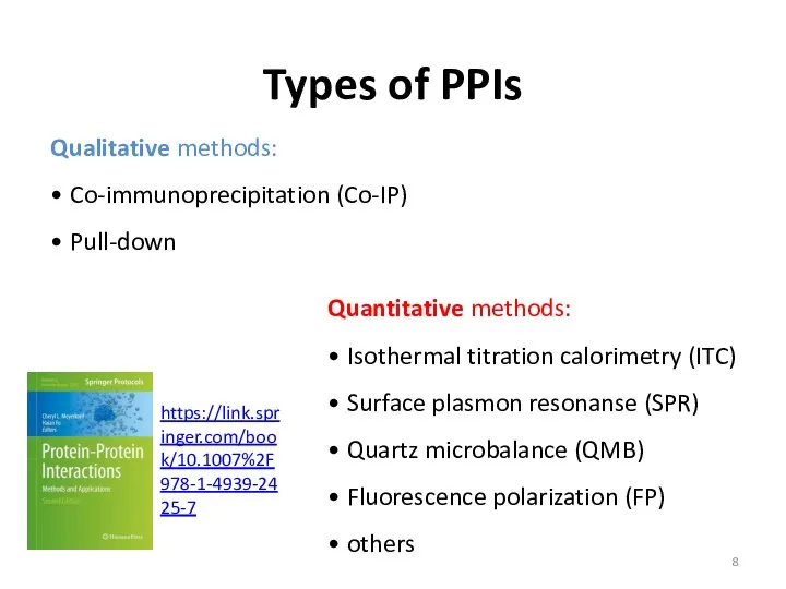
Types of PPIs
Qualitative methods:
• Co-immunoprecipitation (Co-IP)
• Pull-down
Quantitative methods:
• Isothermal titration calorimetry
Types of PPIs
Qualitative methods:
• Co-immunoprecipitation (Co-IP)
• Pull-down
Quantitative methods: • Isothermal titration calorimetry
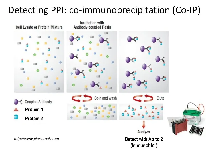
Detecting PPI: co-immunoprecipitation (Co-IP)
Detecting PPI: co-immunoprecipitation (Co-IP)
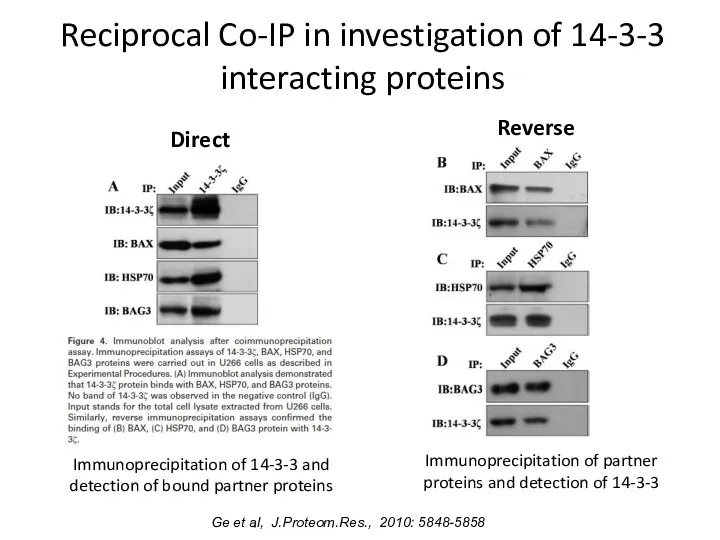
Reciprocal Co-IP in investigation of 14-3-3 interacting proteins
Direct
Immunoprecipitation of 14-3-3 and
Reciprocal Co-IP in investigation of 14-3-3 interacting proteins
Direct
Immunoprecipitation of 14-3-3 and
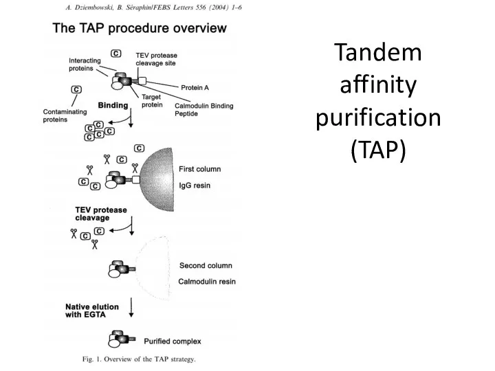
Tandem affinity purification (TAP)
Tandem affinity purification (TAP)
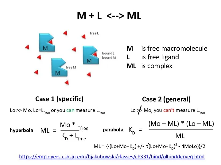
M + L <--> ML
M is free macromolecule
L is free ligand
ML
M + L <--> ML
M is free macromolecule
L is free ligand
ML
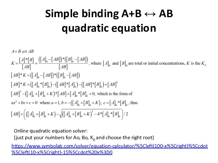
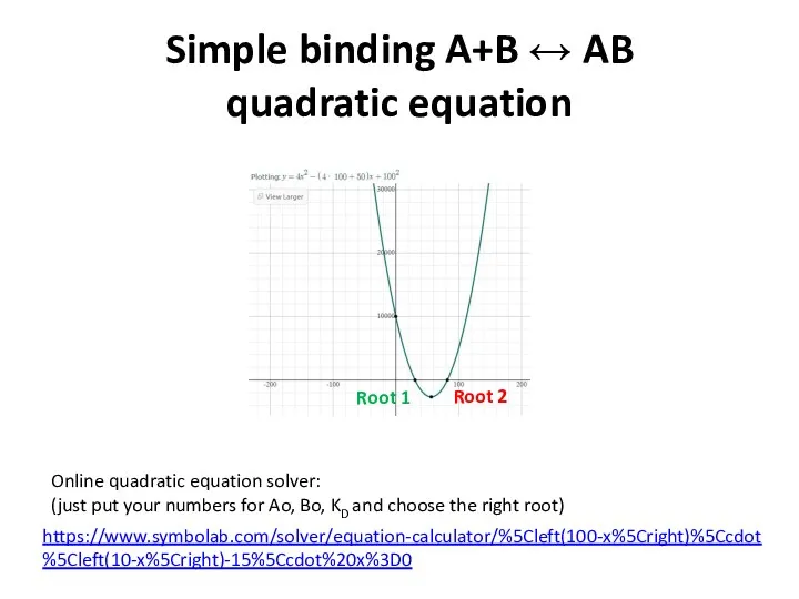
Simple binding A+B ↔ AB
quadratic equation
https://www.symbolab.com/solver/equation-calculator/%5Cleft(100-x%5Cright)%5Ccdot%5Cleft(10-x%5Cright)-15%5Ccdot%20x%3D0
Online quadratic equation solver:
(just
Simple binding A+B ↔ AB
quadratic equation
https://www.symbolab.com/solver/equation-calculator/%5Cleft(100-x%5Cright)%5Ccdot%5Cleft(10-x%5Cright)-15%5Ccdot%20x%3D0
Online quadratic equation solver:
(just
Simple binding A+B ↔ AB
quadratic equation
https://www.symbolab.com/solver/equation-calculator/%5Cleft(100-x%5Cright)%5Ccdot%5Cleft(10-x%5Cright)-15%5Ccdot%20x%3D0
Online quadratic equation solver:
(just
Simple binding A+B ↔ AB
quadratic equation
https://www.symbolab.com/solver/equation-calculator/%5Cleft(100-x%5Cright)%5Ccdot%5Cleft(10-x%5Cright)-15%5Ccdot%20x%3D0
Online quadratic equation solver:
(just
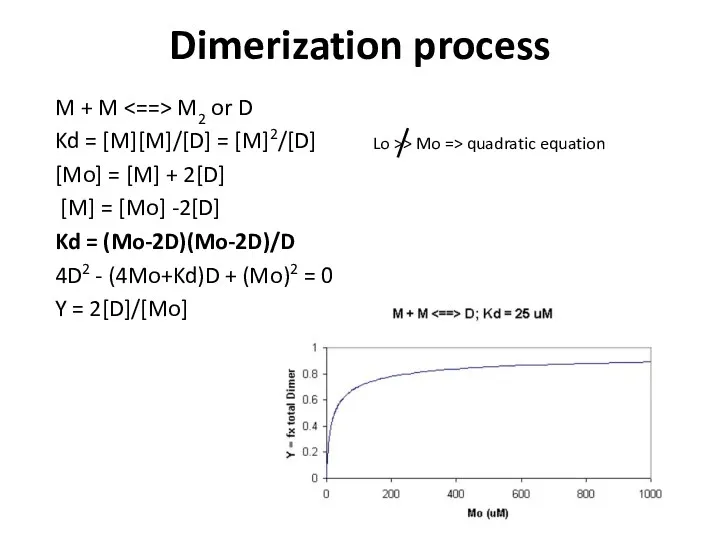
Dimerization process
M + M <==> M2 or D
Kd = [M][M]/[D] =
Dimerization process
M + M <==> M2 or D
Kd = [M][M]/[D] =
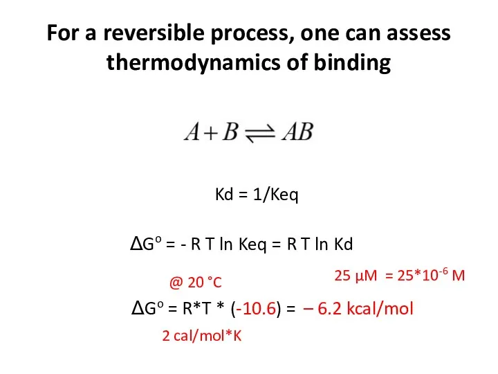
For a reversible process, one can assess thermodynamics of binding
Kd =
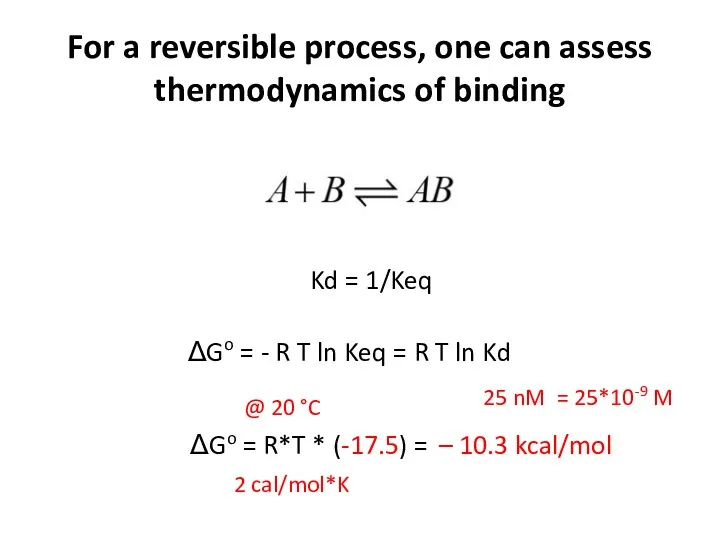
For a reversible process, one can assess thermodynamics of binding
Kd =
For a reversible process, one can assess thermodynamics of binding
Kd =
For a reversible process, one can assess thermodynamics of binding
Kd =
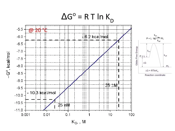
ΔGo = R T ln KD
@ 20 °C
ΔGo = R T ln KD
@ 20 °C
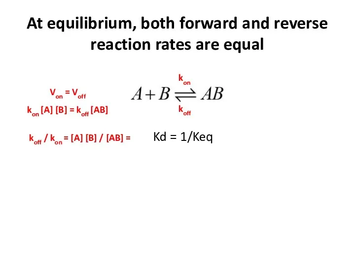
At equilibrium, both forward and reverse reaction rates are equal
Kd =
At equilibrium, both forward and reverse reaction rates are equal
Kd =
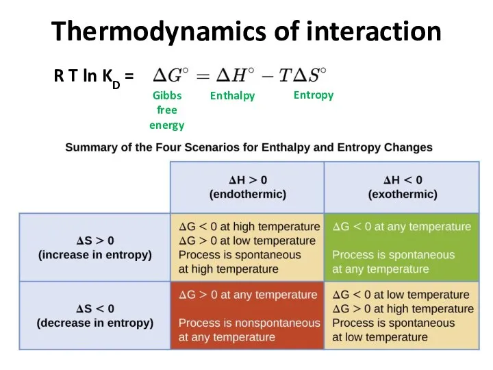
Thermodynamics of interaction
Gibbs free energy
Enthalpy
Entropy
R T ln KD =
Thermodynamics of interaction
Gibbs free energy
Enthalpy
Entropy
R T ln KD =
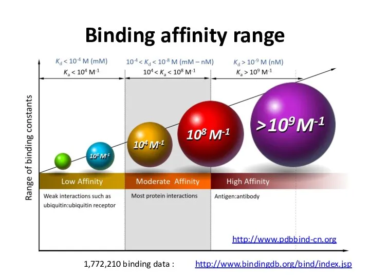
Binding affinity range
http://www.bindingdb.org/bind/index.jsp
1,772,210 binding data :
http://www.pdbbind-cn.org
Binding affinity range
http://www.bindingdb.org/bind/index.jsp
1,772,210 binding data :
http://www.pdbbind-cn.org
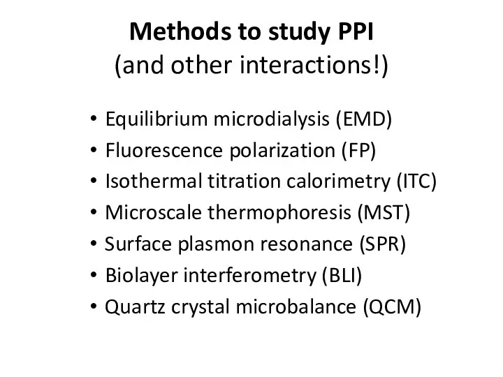
Methods to study PPI
(and other interactions!)
Equilibrium microdialysis (EMD)
Fluorescence polarization (FP)
Isothermal
Methods to study PPI
(and other interactions!)
Equilibrium microdialysis (EMD)
Fluorescence polarization (FP)
Isothermal
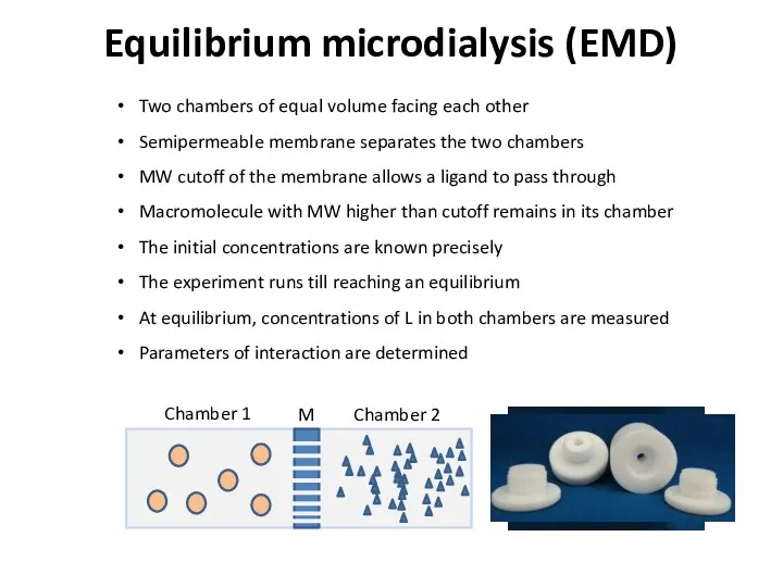
Equilibrium microdialysis (EMD)
Two chambers of equal volume facing each other
Semipermeable membrane
Equilibrium microdialysis (EMD)
Two chambers of equal volume facing each other
Semipermeable membrane
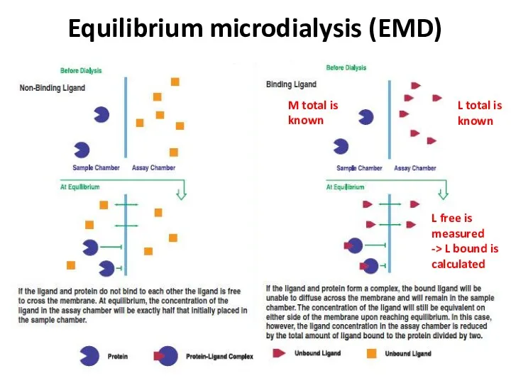
Equilibrium microdialysis (EMD)
L total is
known
L free is measured
-> L bound is
Equilibrium microdialysis (EMD)
L total is
known
L free is measured
-> L bound is
![Equilibrium microdialysis (EMD) KD = [M] * [L] [ML] M](/_ipx/f_webp&q_80&fit_contain&s_1440x1080/imagesDir/jpg/400849/slide-24.jpg)
Equilibrium microdialysis (EMD)
KD =
[M] * [L]
[ML]
M + L <--> ML
Fast
Easy
Inexpensive
Accurate
Equilibrium microdialysis (EMD)
KD =
[M] * [L]
[ML]
M + L <--> ML
Fast
Easy
Inexpensive
Accurate
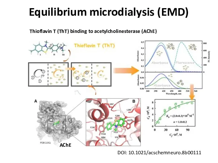
Equilibrium microdialysis (EMD)
DOI: 10.1021/acschemneuro.8b00111
Thioflavin T (ThT) binding to acetylcholinesterase (AChE)
AChE
Equilibrium microdialysis (EMD)
DOI: 10.1021/acschemneuro.8b00111
Thioflavin T (ThT) binding to acetylcholinesterase (AChE)
AChE
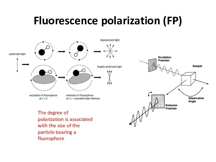
Fluorescence polarization (FP)
The degree of polarization is associated with the size
Fluorescence polarization (FP)
The degree of polarization is associated with the size
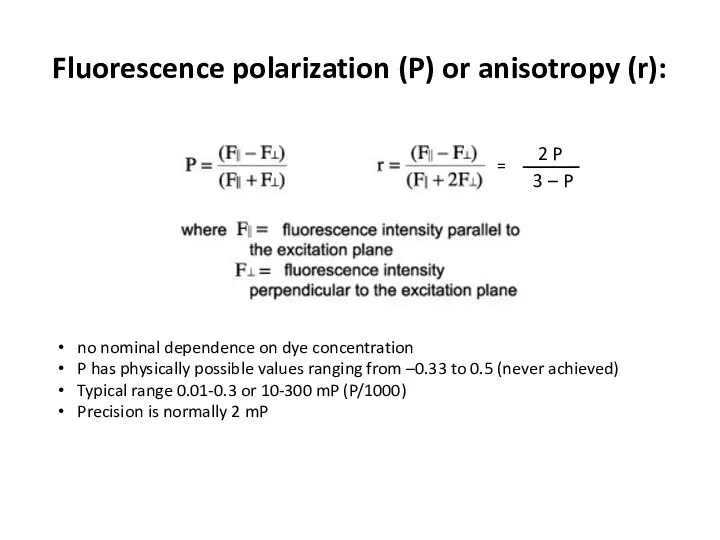
Fluorescence polarization (P) or anisotropy (r):
no nominal dependence on dye concentration
P
Fluorescence polarization (P) or anisotropy (r):
no nominal dependence on dye concentration
P
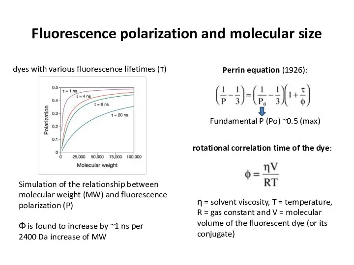
Fluorescence polarization and molecular size
η = solvent viscosity, T = temperature,
Fluorescence polarization and molecular size
η = solvent viscosity, T = temperature,
FP features
Great tool to study interactions
Small sample consumption
Low limit of detection
Rapid
FP features
Great tool to study interactions
Small sample consumption
Low limit of detection
Rapid
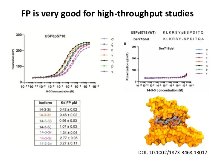
FP is very good for high-throughput studies
DOI: 10.1002/1873-3468.13017
FP is very good for high-throughput studies
DOI: 10.1002/1873-3468.13017
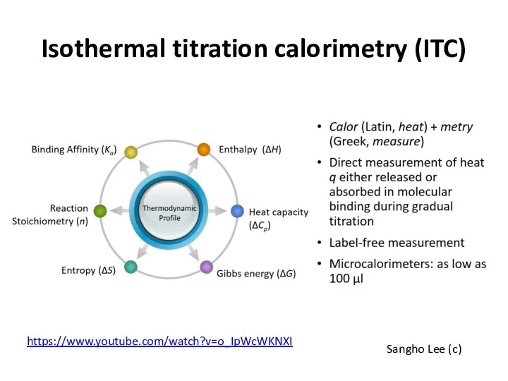
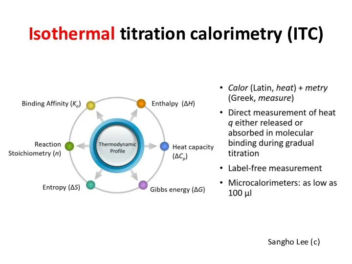
Isothermal titration calorimetry (ITC)
Sangho Lee (c)
https://www.youtube.com/watch?v=o_IpWcWKNXI
Isothermal titration calorimetry (ITC)
Sangho Lee (c)
https://www.youtube.com/watch?v=o_IpWcWKNXI
Isothermal titration calorimetry (ITC)
Sangho Lee (c)
Isothermal titration calorimetry (ITC)
Sangho Lee (c)
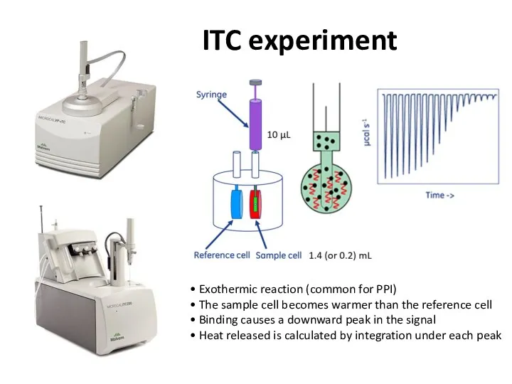
ITC experiment
• Exothermic reaction (common for PPI)
• The sample cell becomes
ITC experiment
• Exothermic reaction (common for PPI)
• The sample cell becomes
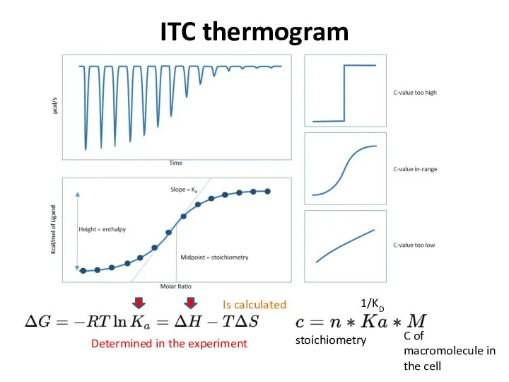
ITC thermogram
stoichiometry
1/KD
C of macromolecule in the cell
Determined in the experiment
Is calculated
ITC thermogram
stoichiometry
1/KD
C of macromolecule in the cell
Determined in the experiment
Is calculated
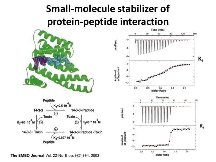
Small-molecule stabilizer of protein-peptide interaction
Small-molecule stabilizer of protein-peptide interaction
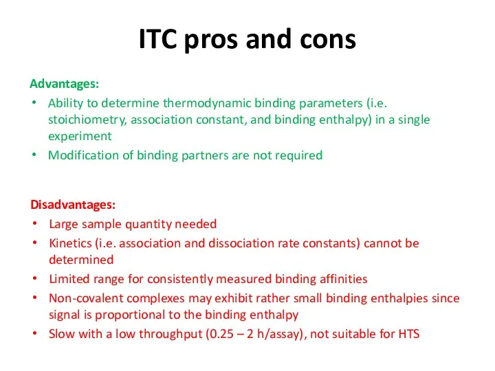
ITC pros and cons
Advantages:
Ability to determine thermodynamic binding parameters (i.e. stoichiometry,
ITC pros and cons
Advantages:
Ability to determine thermodynamic binding parameters (i.e. stoichiometry,
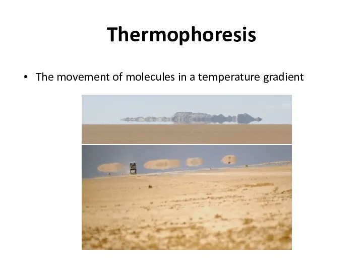
Thermophoresis
The movement of molecules in a temperature gradient
Thermophoresis
The movement of molecules in a temperature gradient
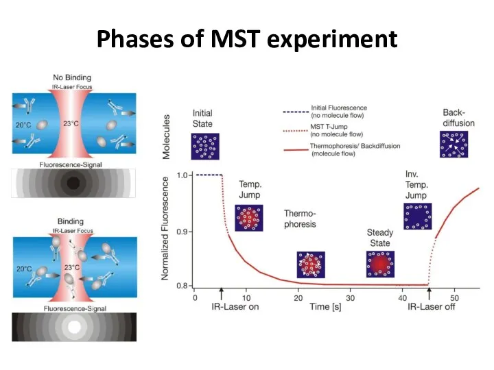
Phases of MST experiment
Phases of MST experiment
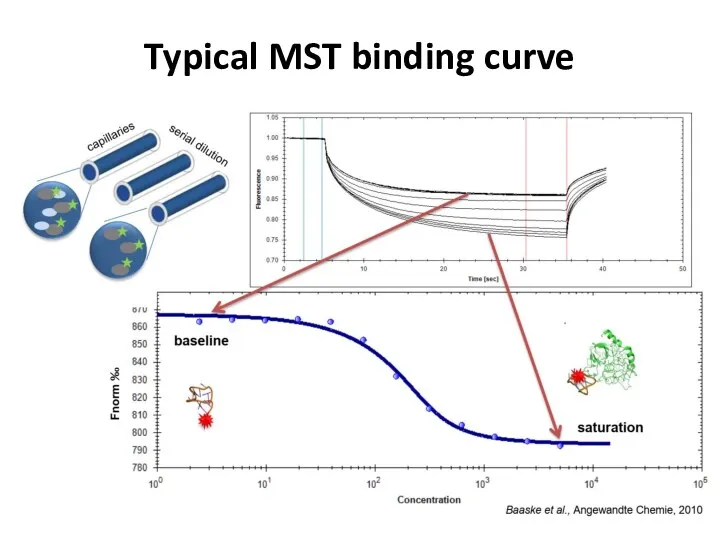
Typical MST binding curve
Typical MST binding curve
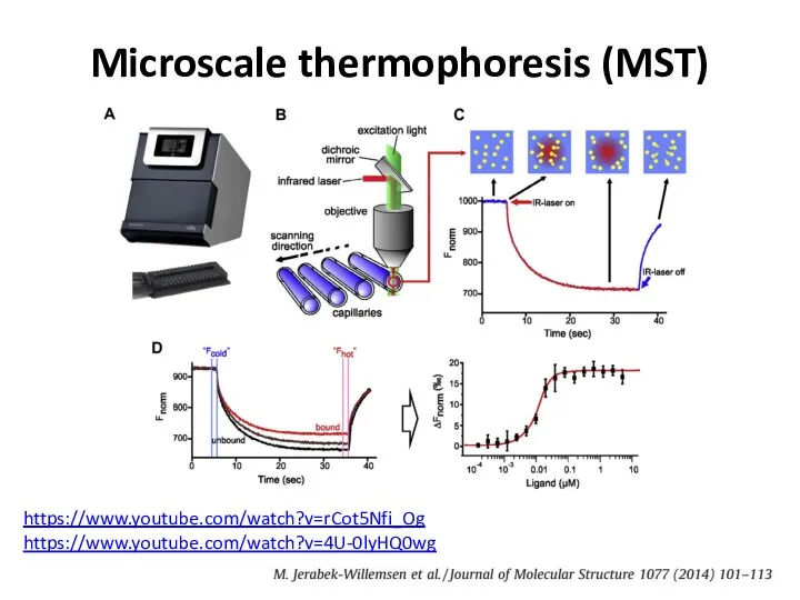
Microscale thermophoresis (MST)
https://www.youtube.com/watch?v=4U-0lyHQ0wg
https://www.youtube.com/watch?v=rCot5Nfi_Og
Microscale thermophoresis (MST)
https://www.youtube.com/watch?v=4U-0lyHQ0wg
https://www.youtube.com/watch?v=rCot5Nfi_Og
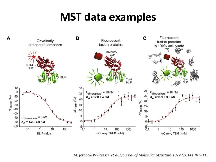
MST data examples
MST data examples
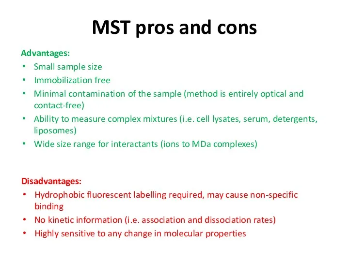
MST pros and cons
Advantages:
Small sample size
Immobilization free
Minimal contamination of the sample
MST pros and cons
Advantages:
Small sample size
Immobilization free
Minimal contamination of the sample
Surface plasmon resonance (SPR)
Surface plasmon resonance (SPR)
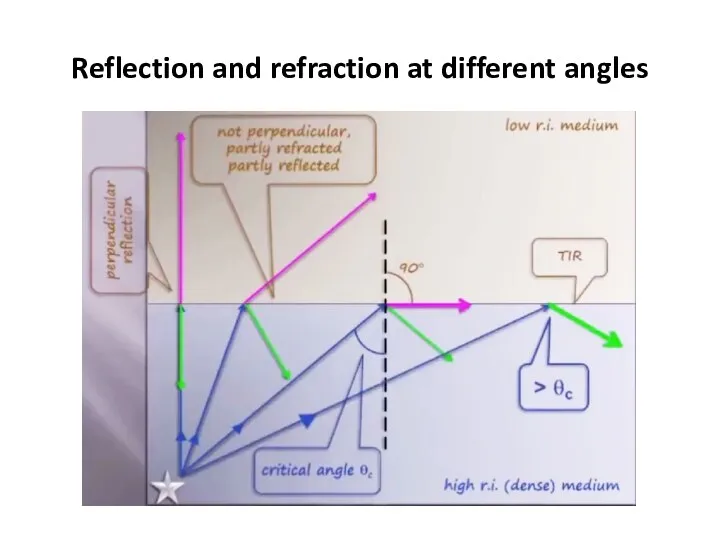
Reflection and refraction at different angles
Reflection and refraction at different angles
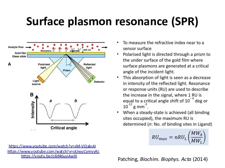
Surface plasmon resonance (SPR)
Patching, Biochim. Biophys. Acta (2014)
https://youtu.be/o8d46ueAwXI
https://www.youtube.com/watch?v=oUwuCymvyKc
https://www.youtube.com/watch?v=sM-VI3alvAI
Surface plasmon resonance (SPR)
Patching, Biochim. Biophys. Acta (2014)
https://youtu.be/o8d46ueAwXI
https://www.youtube.com/watch?v=oUwuCymvyKc
https://www.youtube.com/watch?v=sM-VI3alvAI
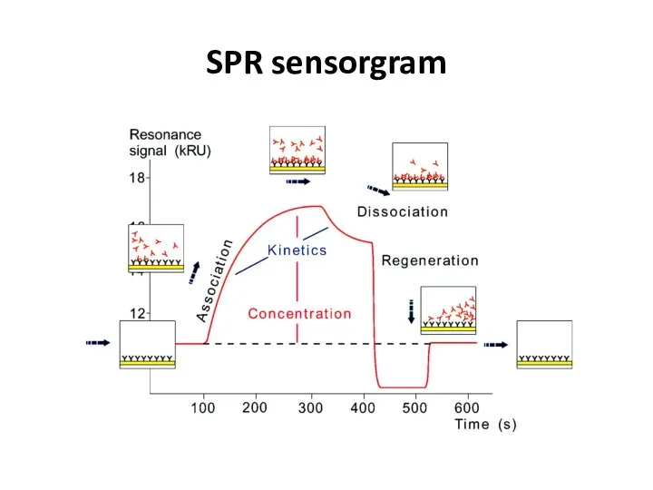
SPR sensorgram
SPR sensorgram
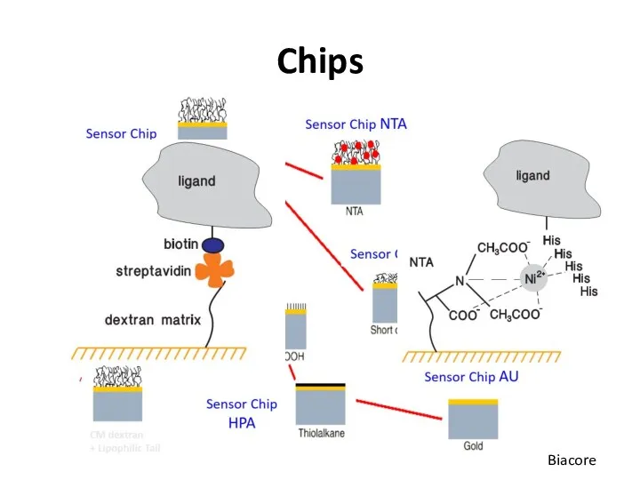
Chips
Biacore
Chips
Biacore
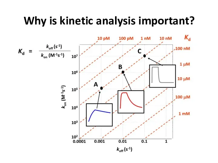
Why is kinetic analysis important?
Why is kinetic analysis important?
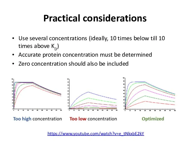
Practical considerations
Use several concentrations (ideally, 10 times below till 10 times
Practical considerations
Use several concentrations (ideally, 10 times below till 10 times
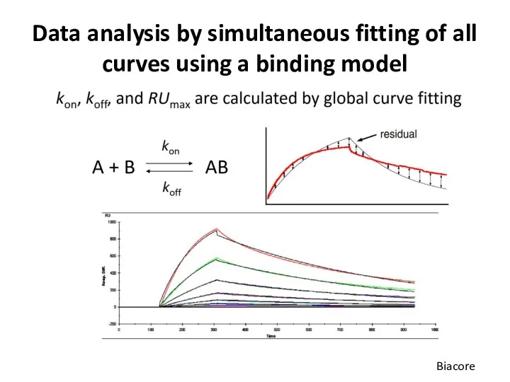
Data analysis by simultaneous fitting of all curves using a binding
Data analysis by simultaneous fitting of all curves using a binding
Steady-state and kinetic ways to determine affinity (KD)
Biacore
Steady-state and kinetic ways to determine affinity (KD)
Biacore

Steady-state and kinetic ways to determine affinity (KD)
Biacore
Steady-state and kinetic ways to determine affinity (KD)
Biacore
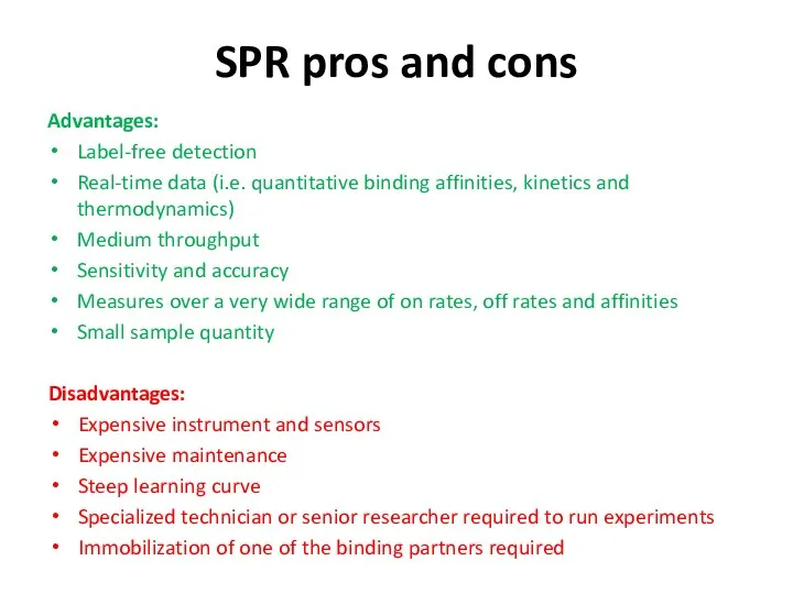
SPR pros and cons
Advantages:
Label-free detection
Real-time data (i.e. quantitative binding affinities, kinetics
SPR pros and cons
Advantages:
Label-free detection
Real-time data (i.e. quantitative binding affinities, kinetics
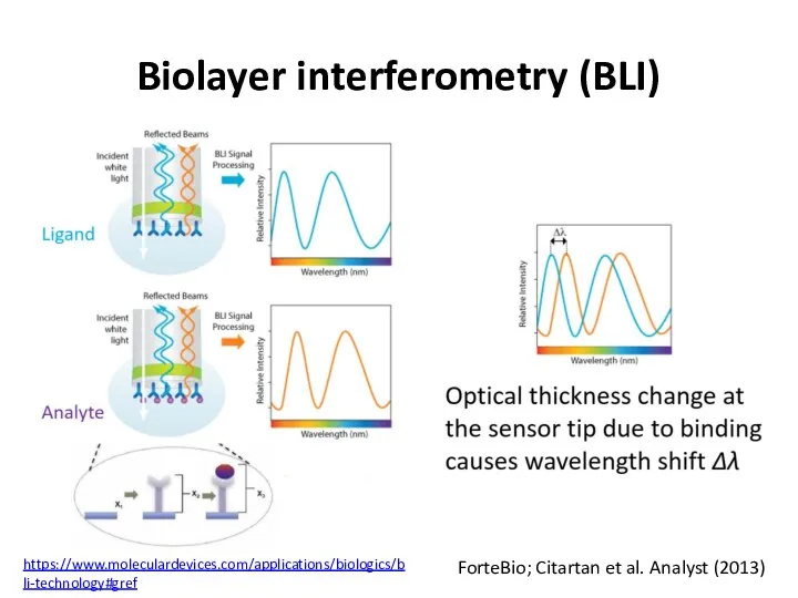
Biolayer interferometry (BLI)
ForteBio; Citartan et al. Analyst (2013)
https://www.moleculardevices.com/applications/biologics/bli-technology#gref
Biolayer interferometry (BLI)
ForteBio; Citartan et al. Analyst (2013)
https://www.moleculardevices.com/applications/biologics/bli-technology#gref
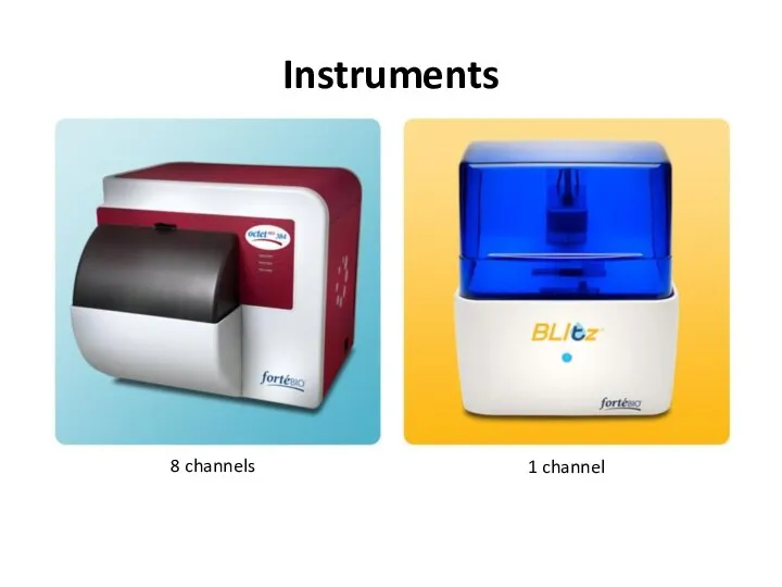
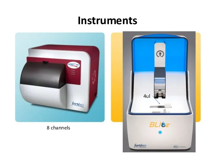
Instruments
8 channels
1 channel
Instruments
8 channels
1 channel
Instruments
8 channels
1 channel
Instruments
8 channels
1 channel
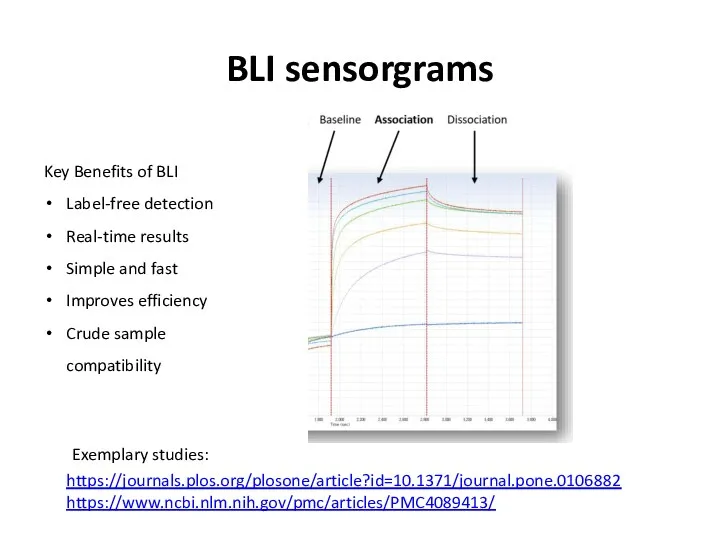
BLI sensorgrams
Key Benefits of BLI
Label-free detection
Real-time results
Simple and fast
Improves efficiency
Crude sample
BLI sensorgrams
Key Benefits of BLI
Label-free detection
Real-time results
Simple and fast
Improves efficiency
Crude sample
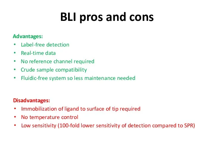
BLI pros and cons
Advantages:
Label-free detection
Real-time data
No reference channel required
Crude sample compatibility
Fluidic-free
BLI pros and cons
Advantages:
Label-free detection
Real-time data
No reference channel required
Crude sample compatibility
Fluidic-free
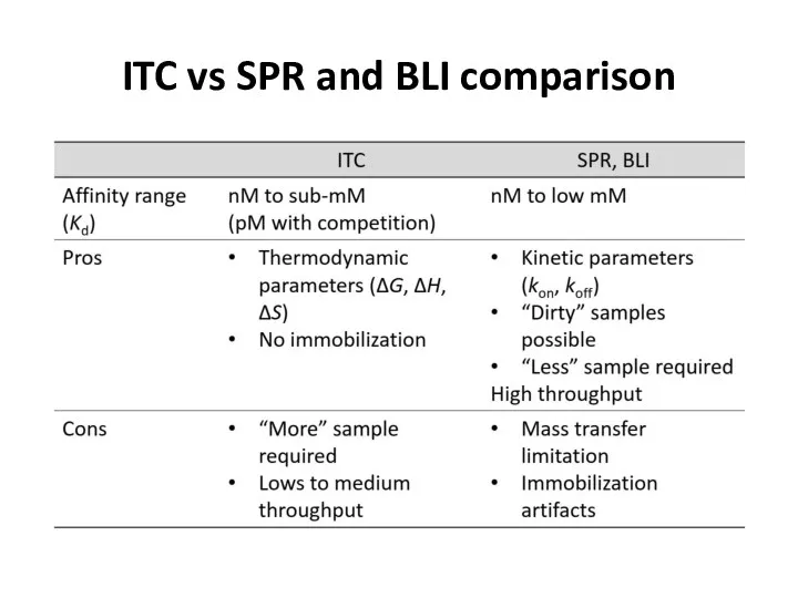
ITC vs SPR and BLI comparison
ITC vs SPR and BLI comparison
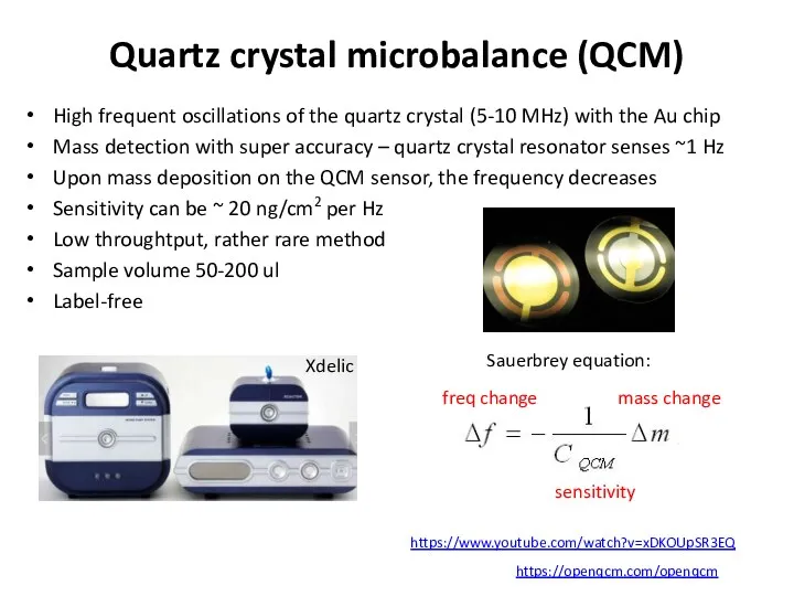
Quartz crystal microbalance (QCM)
High frequent oscillations of the quartz crystal (5-10
Quartz crystal microbalance (QCM)
High frequent oscillations of the quartz crystal (5-10
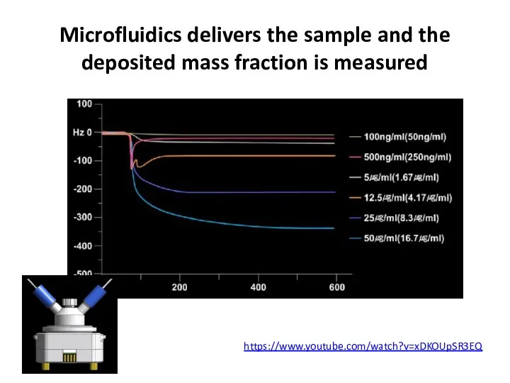
Microfluidics delivers the sample and the deposited mass fraction is measured
Microfluidics delivers the sample and the deposited mass fraction is measured
 Кристаллические решётки и их виды
 Enantioselective Total Synthesis
 Химические свойства солей
 Закон постоянства состава. Молекулярная формула вещества
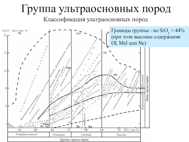 Группа ультраосновных пород
 Строение атома
 Серная кислота
 20230419_izomery
 Бор шикізатын қышқылдық ыдырату
 kremniy
 Алкены. Непредельные углеводороды
 Типы химических реакций. Систематизация и обобщение знаний
 Висмут, ртуть, сурьма
 Метаболизм нуклеиновых кислот
 Методы получения органических галогенидов
 Неметали. Фізичні та хімічні властивості. Явище адсорбції. Сполуки неметалічних елементів з Гідрогеном
 Химия аминокислот. Лекция № 4
 Стратегия химической промышленности
 Вещества
 Химия 20 века
 Газовые смеси
 Правила техники безопасности при работе в химическом кабинете
 Формы парфюмерно-косметической продукции
 Химические свойства основных неорганических соединений в свете ЭД и ОВР. 9 класс
 Создание косметических средств
 Аллотропия. Аллотропные модификации
 Электрохимический ряд напряжений металлов
 Металлы в природе. Способы получения металлов